Download
1 / 29
290 likes | 453 Vues
This document explores various graphical methods for examining data relationships, focusing on single-variable analysis, correlations between two variables, and multidimensional visualizations. Key techniques discussed include histograms, scatterplots, boxplots, 3D visualizations, scatterplot matrices, multivariate profiles, star plots, Andrews' Fourier transformations, metroglyphs, and Chernoff's faces. These techniques enhance the understanding of data distributions and relationships, aiding researchers in identifying patterns and insights from complex datasets.

E N D
Graphical Examination of Data 1.12.1999 Jaakko Leppänen jleppane@cc.hut.fi
Sources • H. Anderson, T. Black: Multivariate Data Analysis,(5th ed., p.40-46). • Yi-tzuu Chien: Interactive Pattern Recognition,(Chapter 3.4). • S. Mustonen: Tilastolliset monimuuttujamenetelmät,(Chapter 1, Helsinki 1995).
Agenda • Examining one variable • Examining the relationship between two variables • 3D visualization • Visualizing multidimensional data
Examining one variable • Histogram • Represents the frequency of occurences within data categories • one value (for discrete variable) • an interval (for continuous variable)
Examining one variable • Stem and leaf diagram (A&B) • Presents the same graphical information as histogram • provides also an enumeration of the actual data values
Examining the relationship between two variables • Scatterplot • Relationship of two variables Linear Non-linear No correlation
Examining the relationship between two variables • Boxplot (according A&B) • Representation of data distribution • Shows: • Middle 50% distribution • Median (skewness) • Whiskers • Outliers • Extreme values
3D visualization • Good if there are just 3 variables • Mustonen: “Problems will arise when we should show lots of dimensions at the same time. Spinning 3D-images or stereo image pairs give us no help with them.”
Visualizing multidimensional data • Scatterplot with varying dots • Scatterplot matrix • Multivariate profiles • Star picture • Andrews’ Fourier transformations • Metroglyphs (Anderson) • Chernoff’s faces
Scatterplot • Two variables for x- and y-axis • Other variables can be represented by • dot size, square size • height of rectangle • width of rectangle • color
Scatterplot matrix • Also named as Draftsman’s display • Histograms on diagonal • Scatterplot on lower portion • Correlations on upper portion
Scatterplot matrix (cont…) correlations histograms scatterplots
Scatterplot matrix (cont…) • Shows relations between each variable pair • Does not determine common distribution exactly • A good mean to learn new material • Helps when finding variable transformations
Scatterplot matrix as rasterplot • Color level represents the value • e.g. values are mapped to gray levels 0-255
Multivariate profiles • A&B: ”The objective of the multivariate profiles is to portray the data in a manner that enables each identification of differences and similarities.” • Line diagram • Variables on x-axis • Scaled (or mapped) values on y-axis
Multivariate profiles (cont…) • An own diagram for each measurement (or measurement group)
Star picture • Like multivariate profile, but drawn from a point instead of x-axis • Vectors have constant angle
Andrews’ Fourier transformations • D.F. Andrews, 1972. • Each measurement X = (X1, X2,..., Xp) is represented by the function below, where - < t < .
Andrews’ Fourier transformations (cont…) • If severeal measurements are put into the same diagram similar measurements are close to each other. • The distance of curves is the Euklidean distance in p-dim space • Variables should be ordered by importance
Andrews’ Fourier transformations (cont…) • Can be drawn also using polar coordinates
Metroglyphs (Andersson) • Each data vector (X) is symbolically represented by a metroglyph • Consists of a circle and set of h rays to the h variables of X. • The lenght of the ray represents the value of variable
Metroglyphs (cont...) • Normally rays should be placed at easily visualized and remembered positions • Can be slant in the same direction • the better way if there is a large number of metrogyphs
Metroglyphs (cont...) • Theoretically no limit to the number of vectors • In practice, human eye works most efficiently with no more than 3-7 rays • Metroglyphs can be put into scatter diagram => removes 2 vectors
Chernoff’s faces • H. Chernoff, 1973 • Based on the idea that people can detect and remember faces very well • Variables determine the face features with linear transformation • Mustonen: "Funny idea, but not used in practice."
Chernoff’s faces (cont…) • Originally 18 features • Radius to corner of face OP • Angle of OP to horizontal • Vertical size of face OU • Eccentricity of upper face • Eccentricity of lower face • Length of nose • Vertical position of mouth • Curvature of mouth 1/R • Width of mouth
Chernoff’s faces (cont…) • Face features (cont…) • Vertical position of eyes • Separation of eyes • Slant of eyes • Eccentricity of eyes • Size of eyes • Position of pupils • Vertical position of eyebrows • Slant of eyebrows • Size of eyebrows
Conclusion • Graphical Examination eases the understanding of variable relationships • Mustonen: "Even badly designed image is easier to understand than data matrix.” • "A picture is worth of a thousand words”