Download
1 / 27
270 likes | 305 Vues
Explore the habitat of the red squirrel in the Mt. Graham area and assess potential impacts of an astronomy observatory construction. Utilize GIS-based modeling, advanced spatial sampling techniques, logistic regression models, trend surface analysis, Bayesian modeling, and habitat loss estimation. Evaluate factors like topography, vegetation, and spatial patterns to determine habitat suitability and quantify potential habitat loss due to construction. Validate models through accuracy assessments and predictive capabilities.

E N D
Environmental Modeling Advanced Weighting of GIS Layers (2)
1. Issue • Modeling the habitat of red squirrel in the Mt. Graham area • Red squirrel prefer a shaded and humid environment and feed on pine cones, that are offered by Mt. Graham • The issue is whether the construction of an astronomy observatory will affect the habitat Pereira, J.M.C., and R.M. Itami, 1991. GIS-based habitat modeling using logistic multiple regression: a study of the Mt. Graham Red Squirrel. Photogrammetric Engineering and Remote Sensing, 57(11):1475-1486.
2. Factors a. Topography: b. Vegetation: Elevation Land cover Slope Canopy closure Aspect (e-w) Food productivity Aspect (n-s) Tree diameter c. Distance to openness (canopy closure and roads)
3. Spatial Sampling • The 200 presence sites are observed in the field • The 200 absence sites can be randomly generated using Hawth’s tool • OR systematically sampled every nth cell, Then n=?
At each of the 400 locations, collect both dependent and the independent variables
3. Spatial Sampling .. • Moran’s I • Cij = 1, if xi and xj are adjacent, Cij=0 otherwise
3. Spatial Sampling .. Moran’s I .. • I = 1 indicates a positive spatial autocorrelation • I = -1 indicates a negative spatial autocorrelation • I = 0 indicates a random spatial pattern
3. Spatial Sampling .. Ileft = 0.94, Imiddle = -1, Iright = 0.168
3. Spatial Sampling .. • The spatial lag can be any value, e.g. 1, 2, 3, 4, …. • When the lag distance increases, the pairs of i and j locations are further apart • The I value decreases with an increasing lag distance, indicating increasing differences between values at i and j locations
3. Spatial Sampling .. • Moran’s I is applied to each variable • lag = 1, 2, 3, … 7 • When lag = 1, I is close to 1 • When lag= 7, I = 0.16 – 0.34 among the ind variables • Every 7th cell is selected • 259 absence cells, compatible to the 212 presence cells
independent variables • Independent variables (14) the continuous variables (1-5, ratio data) 1. Elevation 2. slope 3. aspect (e-w) 4. aspect (n-s) 5. distance to openness (buffer to roads or to land cover)
ind var .. The categorical ind variables 6-14 (nominal, ordinal, or intervaldata) 6-8. Food productivity 9-11. Canopy closure 12-14. Tree diameter
5. Model 1 - the Logistic Model Y = 0.002ele - 0.228slope + 0.685canopy(high) + 0.443canopy(medium) + 0.481canopy(low) + 0.009aspect(e-w) P (Y) = 1/[1 + exp (-Y)] P - The probability of red squirrel habitat
Accuracy Assessment • Error Matrix for the 150 presence and 150 absence sites that are used to develop the logistic model Modeled presence absence total accuracy presence 123 27 150 absence 36 114 150 300 82% Truth 76% Overall accuracy = (123+114)/300 = 79%
Model Validation • Error Matrix for the 50 presence and 50 absence sites that are put aside for model validation Modeled presence absence total accuracy presence 37 13 50 absence 16 34 50 100 74% Truth 68% 71%
5. Model 2 - Trend Surface Analysis • A dependent variable and two independent variables – x and y coordinates • Linear (1st order) : z = a0 + a1x + a2y • Quadratic (2nd order): z = a0 + a1x + a2y + a3x2 + a4xy + a5y2 • Cubic etc. • Least square method
Trends of one, two, and three independent variables for polynomial equations of the first, second, and third orders (after Harbaugh, 1964).
5. Trend Surface Analysis .. • Assuming that the presence and absence depend on coordinates x and y • A 4th order polynomial multiple logistic regression model is used • Dependent variable: presence and absence • Independent variables: x and y • Prediction accuracy: 57%
5. Model 3 - Bayesian Model • A Bayesian model is used to combine the environmental model and the trend surface model • to reach a predictive accuracy of 87%
6. Habitat Loss Estimate • Total number of cells lost to the observatory: Overlay the predicted suitable cells and construction cells • Density of red squirrel in each suitability class: number of presence in the class / acreage of the class • Total habitat loss: S density * acreage per class