Chapter 5 Normal Curve
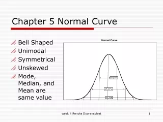
Chapter 5 Normal Curve . Bell Shaped Unimodal Symmetrical Unskewed Mode, Median, and Mean are same value. Theoretical Normal Curve . General relationships: ±1 s = about 68% ±2 s = about 95% ±3 s = about 99%. Theoretical Normal Curve. Using the Normal Curve: Z Scores.

Chapter 5 Normal Curve
E N D
Presentation Transcript
Chapter 5 Normal Curve • Bell Shaped • Unimodal • Symmetrical • Unskewed • Mode, Median, and Mean are same value week 4 Renske Doorenspleet
Theoretical Normal Curve • General relationships: • ±1 s = about 68% • ±2 s = about 95% • ±3 s = about 99% week 4 Renske Doorenspleet
Theoretical Normal Curve week 4 Renske Doorenspleet
Using the Normal Curve: Z Scores • To find areas, first compute Z scores. • The formula changes a “raw” score (Xi) to a standardized score (Z). week 4 Renske Doorenspleet
Using Appendix A to Find Areas Below a Score • Appendix A can be used to find the areas above and below a score. • First compute the Z score, taking careful note of the sign of the score. • Draw a picture of the normal curve and shade in the area in which you are interested. week 4 Renske Doorenspleet
Using Appendix A • Appendix A has three columns. • (a) = Z scores. • (b) = areas between the score and the mean week 4 Renske Doorenspleet
Using Appendix A • Appendix A has three columns. • ( c) = areas beyond the Z score week 4 Renske Doorenspleet
Using Appendix A • Find your Z score in Column A. • To find area below a positive score: • Add column b area to .50. • To find area above a positive score • Look in column c. week 4 Renske Doorenspleet
Using Appendix A • The area below Z = 1.67 is 0.4525 + 0.5000 or 0.9525. • Areas can be expressed as percentages: • 0.9525 = 95.25% week 4 Renske Doorenspleet
Using Appendix A • What if the Z score is negative (–1.67)? • To find area below a negative score: • Look in column c. • To find area above a negative score • Add column b .50 week 4 Renske Doorenspleet
Using Appendix A • The area below Z = - 1.67 is 0.475. • Areas can be expressed as %: 4.75%. • Areas under the curve can also be expressed as probabilities. • Probabilities are proportions and range from 0.00 to 1.00. • The higher the value, the greater the probability (the more likely the event). week 4 Renske Doorenspleet
Finding Probabilities • If a distribution has: • = 13 • s = 4 • What is the probability of randomly selecting a score of 19 or more? week 4 Renske Doorenspleet
Finding Probabilities • Find the Z score. • For Xi = 19, Z = 1.50. • Find area above in column c. • Probability is 0.0668 or 0.07. week 4 Renske Doorenspleet
Finding Probabilities (exercise 1) • The mean of the grades of final papers for this class is 65 and the standard deviation is 5. What percentage of the students have scores above 70? In other words, what is the probability of randomly selecting a score of 70 or more? week 4 Renske Doorenspleet
Finding Probabilities (exercise 2) • Stephen Jay Gould (1996). Full House. The Spread of Excellence from Plato to Darwin. Doctors: you have an aggressive type of cancer and half of the patients will die within 8 months. Question: An optimistic person like Gould was not impressed and not shocked by this message. Why not? week 4 Renske Doorenspleet
Problem: The populations we wish to study are almost always so large that we are unable to gather information from every case. Chapter 6 Introduction to Inferential Statistics : Sampling and the Sampling Distribution week 4 Renske Doorenspleet
Solution: We choose a sample -- a carefully chosen subset of the population – and use information gathered from the cases in the sample to generalize to the population. Basic Logic And Terminology week 4 Renske Doorenspleet
Must be representative of the population. Representative: The sample has the same characteristics as the population. How can we ensure samples are representative? Samples in which every case in the population has the same chance of being selected for the sample are likely to be representative. Samples week 4 Renske Doorenspleet
Sampling Techniques • Simple Random Sampling (SRS) • Systematic Random Sampling • Stratified Random Sampling • Cluster Sampling • See Healey’s book for more information on differences between those techniques week 4 Renske Doorenspleet
Applying Logic and Terminology • For example: • Population = All 20,000 students. • Sample = The 500 students selected and interviewed week 4 Renske Doorenspleet
Every application of inferential statistics involves 3 different distributions. Information from the sample is linked to the population via the sampling distribution. The Sampling Distribution Population Sampling Distribution Sample week 4 Renske Doorenspleet
First Theorem • Tells us the shape of the sampling distribution and defines its mean and standard deviation. • If we begin with a trait that is normally distributed across a population (IQ, height) and take an infinite number of equally sized random samples from that population, the sampling distribution of sample means will be normal. week 4 Renske Doorenspleet
Central Limit Theorem • For any trait or variable, even those that are not normally distributed in the population, as sample size grows larger, the sampling distribution of sample means will become normal in shape. week 4 Renske Doorenspleet
The Sampling Distribution: Properties • Normal in shape. • Has a mean equal to the population mean. • Has a standard deviation (standard error) equal to the population standard deviation divided by the square root of N. The Sampling Distribution is normal so we can use Appendix A to find areas. See Table 6.1, p. 160 of Healey’s book for specific important symbols. week 4 Renske Doorenspleet