Angle Modulation
Angle Modulation. Professor Z Ghassemlooy Electronics & IT Division Scholl of Engineering Sheffield Hallam University U.K. www.shu.ac.uk/ocr. Contents. Properties of Angle (exponential) Modulation Types Phase Modulation Frequency Modulation Line Spectrum & Phase Diagram

Angle Modulation
E N D
Presentation Transcript
Angle Modulation Professor Z Ghassemlooy Electronics & IT Division Scholl of Engineering Sheffield Hallam University U.K. www.shu.ac.uk/ocr Z. Ghassemlooy
Contents • Properties of Angle (exponential) Modulation • Types • Phase Modulation • Frequency Modulation • Line Spectrum & Phase Diagram • Implementation • Power Z. Ghassemlooy
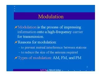
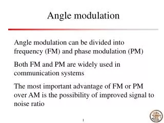
Properties • Linear CW Modulation (AM): • Modulated spectrum is translated message spectrum • Bandwidth message bandwidth • SNRoat the output can be improved only by increasing the transmitted power • Angle Modulation: A non-linear process:- • Modulated spectrum is not simply related to the message spectrum • Bandwidth >>message bandwidth. This results in improved SNRowithout increasing the transmitted power Z. Ghassemlooy
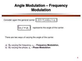
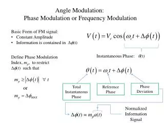
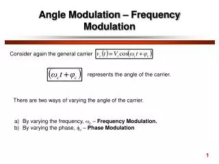
Basic Concept • First introduced in 1931 A sinusoidal carrier signal is defined as: For un-modulated carrier signal the total instantaneous angle is: Thus one can express c(t) as: • Thus: • Varying the frequency fc Frequency modulation • Varying the phase c Phase modulation Z. Ghassemlooy
c(t) (red) Unmodulated carrier Frequency-modulated angle 47/2 Unmodulated carrier 35/2 Phase-modulated angle Amplitude Ec 23/2 11/2 -/2 Slope =c/t t (ms) Initial phasec 0 1 2 4 3 t t = 0 m(t) 2 0 -1 Basic Concept - Cont’d. • In angle modulation: Amplitude is constant, but angle varies (increases linearly) with time Z. Ghassemlooy
i(t) Ec c(t) c(t) c(t) Phase Modulation (PM) PM is defined If Thus Where Kp is known as the phase modulation index Instantaneous phase Instantaneous frequency Rotating Phasor diagram Z. Ghassemlooy
Frequency Modulation (FM) The instantaneous frequency is; Where Kf is known as the frequency deviation (or frequency modulation index). Note: Kf < fc to make sure that f(t) >0. Instantaneous phase Note that Integrating Substituting c(t) in c(t) results in: Z. Ghassemlooy
Waveforms Z. Ghassemlooy
75 kHz, FM Radio, (88-108 MHz band) 25 kHz, TV sound broadcast 5 kHz, 2-way mobile radio 2.5 kHz, 2-way mobile radio FD = Important Terms • Carrier Frequency Deviation (peak) • Frequency swing • Rated System Deviation (i.e. maximum deviation allowed) • Percent Modulation • Modulation Index Z. Ghassemlooy
Since and FM Spectral Analysis Let modulating signal m(t) = Em cos mt Substituting it in c(t)FM expression and integrating it results in: the terms cos ( sin mt) and sin ( sin mt) are defined in trigonometric series, which gives Bessel Function Coefficient as: Z. Ghassemlooy
Bessel Function Coefficients cos ( sin x) = J0 () + 2 [J2() cos 2x + J4() cos 4x + ....] And sin ( sin x) = 2 [J1() sin x + J3() sin 3x + ....] where Jn() are the coefficient of Bessel function of the 1st kind, of the order n and argument of . Z. Ghassemlooy
FM Spectral Analysis - Cont’d. Substituting the Bessel coefficient results in: Expanding it results in: Carrier signal Side-bands signal (infinite sets) Since Then Z. Ghassemlooy
J0() Side bands J1() J4() J2() J2() J3() J4() c- 3m c- 4m c- 2m c+ m c+ 3m J3() c c+ 2m c+ 4m Side bands FM Spectrum Bandwidth (?) Z. Ghassemlooy
= 2.5 = 0.5 = 1.0 = 4 c c c c Bandwidth FM Spectrum - cont’d. • The number of side bands with significant amplitude depend on • see below Most practical FM systems have 2 < < 10 Generation and transmission of pure FM requires infinite bandwidth, whether or not the modulating signal is bandlimited. However practical FM systems do have a finite bandwidth with quite well pwerformance. Z. Ghassemlooy
FM Bandwidth BFM • The commonly rule used to determine the bandwidth is: • Sideband amplitudes < 1% of the un-modulated carrier can be ignored.Thus Jn()> 0.01 BFM = 2nfm= 2fm=2 (fc/ fm).fm = 2 fc For large values of , For small values of , BFM = 2fm For limited cases General case: use Carson equation BFM 2(fc + fm) BFM 2 fm (1 + ) Z. Ghassemlooy