EDAX Operation
EDAX Operation. Operation of the Phoenix EDAX system Basic information on EDS analysis Introduction to Mapping, Line scans, and OIM or EBSD. Set the EDS parameters according to the type of analysis needed. Use the SETUP Menu to select the time. Set up SEM. Column set up to Analysis mode

EDAX Operation
E N D
Presentation Transcript
EDAX Operation • Operation of the Phoenix EDAX system • Basic information on EDS analysis • Introduction to Mapping, Line scans, and OIM or EBSD
Set the EDS parameters according to the type of analysis needed. Use theSETUPMenu to select the time.
Set up SEM • Column set up to Analysis mode • Area of interest selected • Column and aperture aligned • Analysis Scan Mode selected • Condenser Lens 1 set • Dead time at ~32% • CPS above 1000
To collect a spectrum set the SEM on the area or point of interest. Use the second menu button (paint-roller) to clear the screen of the previous spectrum. Click the first menu button (stop watch) to acquire a spectrum.
Once the spectrum is acquired use thePeak Identificationcontrol panel by clicking on“AUTO”to label the peaks present. To remove a element, select the element from the“Saved Elem”list box and click the “Delete” button
Add an element: • Typing four characters(SiKa or AgLa)“Element”box. • Select an element that is near the element you want to add and click“Z- or Z+” • Click the cursor on the peak to identify, then click the choice from the“Pos Elem”box
Once the spectrum has been labeled click on the “File” and “Save”. The file can be saved as the raw data or as an image of the spectrum. A saved spectrum will no longer be able to be manipulated. All data is to be saved on the D drive and will be periodically removed.
Auto acquisition of spectrums Auto quantify spectrums Auto identify spectrums Compare spectrums Returns the spectrum to original state Reduces the height of the spectrum Increases the height of the spectrum Shrinks the spectrum in the X direction Expands the spectrum
If the“Dead time”is to high or not high enough and you have checked the SEM parameters then you can change the“AMP Time”in the“EDAM”control box
If the back ground is off for your spectrum you can change the parameters from Auto to Manual or from Manual to Auto. In Manual you have the ability to add or delete specific points along the spectrum for a better background fit.
After the spectrum is saved do a deconvolution fit on the spectrum. This is done with the HPD (Halographic Peak Deconvolution) button in Peak Identification control window. The deconvolution shows up as line across the very top of the spectrum (red). A background will also show up as a line on the bottom of the spectrum (blue). This will allow you to see if the software will correctly quantify the spectrum. BackgroundDeconvolution Cursor
If deconvolution does not follow the top of the peaks use theEPICtable in thePeak Identificationwindow to adjust the specific element parameters
When the deconvolution and background are correct the spectrum can be quantified. Either select the“Quantify”control panel or theAuto Quantify button. In the“Quantify”control panel there are options to adjust the quantification of the spectrum. For general purposes these are not necessary.
Use the“Quantify”button at the bottom to analyze the spectrum. Once done a“Results”box will appear. You can show only one result or multiple results. These can be printed or saved and imported to an Excel file.
Elemental Mapping A system creates an elemental map based on ROI (region of interest).
Elements of interest are defined in the software. Counts are collected from that region of the spectra and mapped. Each pixel intensity is relative to the concentration of that element. Elements are given different colors for easier viewing. Higher counts have better results.
Collecting x-ray data from a number of points along a preselected line.
EDS Summary • Signal comes from interaction volume • Features of < 1um will have matrix information in the spectra • Don’t coat with element of interest • Count times should be long enough to discern low concentrations from background