Download
1 / 16
160 likes | 273 Vues
Explore electron optics nonlinearity using YAG images, differential orbit measurements, and nonlinearity coefficients. Hypothesize main sources, test theories with bump data, and optimize optics for linearity.

E N D
Linearity of the Electron Optics Alexey Burov RR Talks
Examples of YAG images • In many cases, YAG images of e-beam had distinct triangular shape, • pointing to a sextupole nonlinearity (Sasha, Lionel). • This nonlinearity has to be seen in differential orbit measurements. • The differential orbit measurements were done by Mary: • A5 & A6 correctors Oct 29 (not clean in CS) , Nov 6 (OK for CS); • S2 & S5 - Nov 1; • S3 – Nov 26; S4 – Nov 29.
Nonlinearity Coefficient • For every mentioned corrector, 10 equidistant kicks were applied, from the highest possible negative, to the highest positive. For every corrector j, the BPM data were saved in P163 format. • To see nonlinearity in these data, I prepared a MathCad file, which makes a linear fit for every given BPM i , and subtract this fit from the data • For every BPM i, the nonlinearity is characterized by • For every corrector, the measure of nonlinearity of its trajectories can be presented as
Example for CXA05 BXS05, cm BYS05, cm
Results The numbers are not negligible. Currently, the angle is estimated ~ 100μrad on the axis. Nonlinearities for below CS2 are small. Also: nonlinearities for BS2, BS3 were always small (not shown here). Max nonlinearity are always at XC4, YC8 ( ≈ π/2 of the Larmor phase). Hypothesis: The main source of nonlinearity is located at the lens S3
Accuracy (CYS2 kicks) Error of CYS2 current (or is it MI perturbation?) is equivalent to 100-200 microns of the bpm error. And this case is not unique… How can we avoid this?
How to check the hypothesis • To check the SS3 hypothesis, a local bump CYS2-CYS3-CYS4 can be done. • Then, for several bump mults, bpm data can be taken and compared with the nonlinear parts of Nov 1 CYS2 measurements. • Nov 1 CYS2 & CXS2 measurements should be redone, due to their high errors for some points.
Cylindrical Aberrations of Ideal Lens • Focusing strength of a solenoid can be derived as: • Assuming • In local bumps, this nonlinearity has to be seen as a cubic parabola in a plane of the bump, and ~nothing in the other plane, as soon as the lens is optically thin. • For
Bump nonlinearity • For a linear local 3-bump around a doublet • A nonlinear offset in the bpm BS4 , for SS3 + - BS4 BS3 CS2 CS3 CS4
Cx/yS2 Bump Data CYS2 bump CXS2 bump Huge nonlinearity of SS3! 14%/2.5%=6 times of the ideal level
CS2 bumps show: • Nonlinearities seen in these bumps: • None of them has symmetry of the solenoidal lens • Y-bump is ~ 3 times more nonlinear as X-bump (as in P163, p.5) • Absolute value of Y-bump nonlinearity is 5 times higher the ideal level (also agrees with the P163 data in p.5). • Dependences of BS3(CS2) are all linear at the noise level. • Thus, these bump data confirm my hypothesis about extremely nonlinear S3 lens
CS3 bump CYS3 bump CXS3 bump Nonlinearity of SS4 is 5%/2.5% = 2 times of the ideal level.
Lens T4 • The same way of measurements with the 3-bump around ST4 (Mary, 08Feb21_linearity measurement) yields non-linearity as 4 times of the ideal level.
Conclusions • Bump measurements give the same ratios of nonlinearities as P163. • The hypothesis of extreme SS3 nonlinearity (6 times more than natural , 3 times more than SS4) is confirmed. • Other measured lenses have following nonlinearities: • SS4: 2 times of the natural level • ST4: 4 times of the natural level • It is reasonable to explore the most linear part for the beam position in SS3 (~-5 mm), and to optimize optics, reducing the field in SS3.