Linearity of the BOLD Response
Linearity of the BOLD Response. Peter A. Bandettini Rasmus Birn Ziad Saad Dan Kelley Unit on Functional Imaging Methods Laboratory of Brain and Cognition, National Institute of Mental health, NIH. Hemodynamic Transfer Function. Neuronal. Measured. Activation. fMRI. Signal.

Linearity of the BOLD Response
E N D
Presentation Transcript
Linearity of the BOLD Response Peter A. Bandettini Rasmus Birn Ziad Saad Dan Kelley Unit on Functional Imaging Methods Laboratory of Brain and Cognition, National Institute of Mental health, NIH
Hemodynamic Transfer Function Neuronal Measured Activation fMRI Signal Hemodynamics Physiolologic Factors
Motor Cortex Auditory Cortex
2 1000 msec 1.5 100 msec 34 msec 1 0.5 0 -0.5 -1 15 20 25 30 35 Time (sec) Savoy et al.
Methods Motor Visual Stimulus Duration (SD) … SD = 500 ms SD = 250 ms … SD = 1000 ms SD = 500 ms … SD = 2000 ms SD = 1000 ms … SD = 4000 ms SD = 2000 ms 16 s … Blocked Trial 20 s
Observed Responses measured ideal (linear) visual stimulation 250 ms 500 ms 1000 ms 2000 ms motor task 500 ms 1000 ms 2000 ms 4000 ms
20 s 2000 ms 1000 ms 500 ms 250 ms 0 10 20 30 40 0 10 20 30 40 BOLD response is nonlinear Observed response Linear response Short duration stimuli produce larger responses than expected
20, 20 12, 2 10, 2 8, 2 6, 2 4, 2 2, 2 Contrast to Noise Images ( ISI, SD ) S1 S2
Source of the Nonlinearity • Neuronal • Hemodynamic • Miller et al. 1998 – Flow is linear, BOLD is nonlinear • Friston et al. 2000 – hemodynamics can explain nonlinearity If nonlinearity is hemodynamic in origin, a measure of this nonlinearity will reflect any spatial variation of the vasculature
a t Compute nonlinearity (for each voxel) • Amplitude of Response Fit ideal (linear) to response • Area under response / Stimulus Duration Output Area / Input Area
6 6 4 f (SD) 4 f (SD) 2 2 0 1 2 3 4 5 0 1 2 3 4 5 Stimulus Duration Stimulus Duration 6 5 4 4 3 2 2 1 0 1 2 3 4 5 0 1 2 3 4 5 Nonlinearity Visual Motor Magnitude linear Area Output / input Output / input Stimulus Duration Stimulus Duration
Results – visual task Nonlinearity Magnitude Latency
Results – motor task Nonlinearity Magnitude Latency
8 f (SD) 6 4 2 0 10 20 30 40 0 1 2 3 4 5 0 10 20 30 40 Stimulus Duration -2 8 f (SD) 6 60 4 40 2 20 0 1 2 3 4 5 0 2 0 2 4 6 8 Stimulus Duration -2 nonlinearity Results – visual task
8 f (SD) 6 4 2 60 0 10 20 30 40 0 10 20 30 40 40 0 1 2 3 4 5 Stimulus Duration 20 0 2 0 2 4 6 8 nonlinearity Results – motor task 8 f (SD) 6 4 2 0 1 2 3 4 5 Stimulus Duration
Reproducibility Visual task Motor task Nonlinearity1 Nonlinearity1 Nonlinearity2 Nonlinearity2 Experiment 1 Experiment 2 Experiment 1 Experiment 2
time (s) Different stimulus “ON” periods measured linear BOLD Response Signal Stimulus timing 0.25 s 0.5 s 1 s 2 s 20 s Brief stimuli produce larger responses than expected
time (s) Different stimulus “ON” periods measured BOLD Response Signal linear Stimulus timing 2 s 3 s 4 s 8 s 16 s Brief stimulus OFF periods produce smaller decreases than expected
Varying “ON” and “OFF” periods • Rapid event-related design with varying ISI 8% ON 25% ON 50% ON 75% ON
8% ON Measured Blocked Response 8% ON 25% ON 50% ON 25% ON Signal 50% ON 75% ON 75% ON Signal 0 10 20 30 40 0 5 15 10 time (s) time (s) Varying “ON” and “OFF” periods Estimated Impulse Response Predicted Responses to 20 s stimulation
Conclusions • For brief stimulus “ON” periods, signal increases are larger than expected. These nonlinearities show considerable yet reproducible spatial heterogeneity. • For brief stimulus “OFF” periods, signal decreases are smaller than expected • For varying “ON” and “OFF” periods, deconvolved impulse response depends on fraction of time in “ON” state.
Sources of this Nonlinearity • Neuronal • Hemodynamic • Oxygen extraction • Blood volume dynamics Oxygen Extraction Flow In Flow Out D Volume
BOLD Curves A Linear and Nonlinear “Balloon” BOLD Curves for Varying SD 20,2,1,0.5, 0.25 sec B Balloon Curves, SD = 20 sec: One parameter is varied at a time. When not varied they are set equal to V0 = 0.03, E0 = 0.3, and Gam = 2.6 C Balloon Curves, SD = 2 sec: One parameter is varied at a time. When not varied they are set equal to V0 = 0.03, E0 = 0.3, and Gam = 2.6 A B C
Dilution Effects Increase FlowIn > Flowout Washout Effects Increase FlowOut > FlowIn Balloon Model Parameters For a given flow of blood into the venous compartment, the three Balloon parameters which control the hemodynamic contribution to the BOLD signal are thought to be E0, V0, and Gam. E0 represents thefraction of total hemoglobin not bound to O2; v(t) is the fraction of voxel volume filled with blood during the active state normalized to that at rest, V0; o is the mean venous transit timeof blood in the venous compartment and equals V0 / FlowOut(0); Gam is the exponent defining the relationship between venous outflow and fractional blood volume; q(t) is the total voxel content of dHB during the active state normalized to that at rest; viscos is a viscosity term that varies between viscup, during balloon inflation, and viscdown, during balloon deflation. On a voxelwise basis, the stimulus waveform was smoothed (WAVrisetime), scaled (FLINamp), and phase shifted (FLINdelay) in order to generate an optimally fitting curve, ShiftedFlowIn(t), representing blood flow into the venous compartment.
64.29 Gam = 0 0.01 Vo 0.05 0.1 Eo 0.5 0 1.644 Gam 6.516 Gam = 2 8 5.683 6.437 Gam = 2.6 5.691 7.267 Gam = 4 6.250 7.512 Gam = 6 6.465 7.612 Gam = 8 6.537 Balloon Model Nonlinearity Maps Area Under f(SD) vs. Gam E0 = 0.3 ; V0 = 0.03 E0, dHb fraction; V0, blood volume fraction at rest; Gam, steady state venous outflow-volume relationship o , the mean venous transit timeof blood; Physiological Parameter Contribution to NL Gam << 2 Gam >> (o > E0) 2 << Gam << 4 o >> (E0> Gam) Gam 4 (o E0) >> Gam 4<< Gam < 8 E0>> (o > Gam) Main NL dependence Gam << 2 v(t) and FlowOut(t) NL Range >> 1 Larger NLSmaller NL o Shorter Longer E0 Larger Smaller Gam >= 2o and E0NL Range 1 Larger NLSmaller NL o Longer Shorter E0 Smaller Larger
For TE = 30ms 1.5T3.0T k1 5.2 * E0 10.4 * E0 k2 1.43 * E0 0.5 * E0 k3 0.43 -0.5 Figure 2: Balloon Curves at different Tesla, SD = 20 sec. V0 = 0.03, E0 = 0.3, and Gam = 2.6
Conclusions When varied independently, E0, V0, and Gam each affect the BOLD signal in different ways. The interaction of these parameters produces BOLD curves that are nonlinear when compared to the linear results using the same SD. For Gam values between 0 and 2, in which venous outflow is not laminar, small increases in Gam reduce nonlinearity (NL). Nonlinearity is a function of several parameters, whose relative contributions to NL are determined by the value of each parameter. For Gam values between 2.1 to 6.4 and with other parameters in physiological range, NL values ranged from 6.01 to 7.53. By limiting the NL range to the range of NL obtained experimentally ( NL between 5 and 10), the balloon model can be further constrained in our attempt to extract physiologic information from the BOLD response in humans. Further analysis is necessary to determine how varying the viscoelasticity of the venous compartment affects NL.
Balloon Model Parameter Estimation Relevant Physiologic Range E0 0.2 to 0.4 V0 0.02 to 0.05 Gam 2.1 to 6.4
Entire Averaged Run Epochs in Averaged Run Stimulus A Stimulus B Stimulus A Stimulus B Magnitudes of Averaged Raw Data Magnitudes of Averaged Balloon Model Fit Raw Experimental Data versus the Optimal Balloon Model Fit The magnitudes for different stumuli (A and B), averaged across two runs, are plotted for epochs (16, 4, 2, 1 sec) within an averaged run and for all epochs in the averaged run).
Conclusions Balloon model hemodynamics do not fully account for human BOLD signal NL. Within a run for a given stimulus, epochs of longer stimulus duration are better characterized by the Balloon model than shorter stimulus durations. As epoch durations become briefer, the Balloon model fits become more linear relative to experimental data.