Download
1 / 57
650 likes | 958 Vues
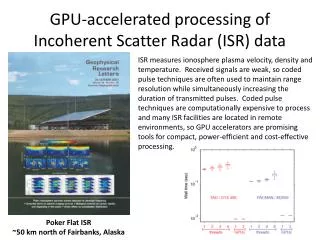
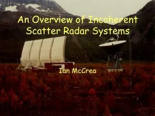
An Overview of Incoherent Scatter Radar Systems. Ian McCrea. RADAR. acronym for RAdio D etection A nd R anging:

E N D
RADAR • acronym forRAdioDetection And Ranging: • Generic name for measuring systems deriving information about distant objects (radar targets) by illuminating them with RF energy and recording the reflected and/or back-scattered energy, • In the early days, only the presence of, and range to, the radar targets could be inferred, (that is how the acronym became RADAR...) • Today, many radar systems also allow spectral analysis and (sometimes) target imaging.
A generic radar system Radar target: Physics Engineering Receiving antenna: Ar Transmitting antenna: GT Power: P To computer TX RX A/D Signal generator Timing & Control
t t’ p(t) z(t)z(t’) Z=(p*e) Correlator Lag Profiles Receiver An Idealised Radar System env(t) e(t)
How do Incoherent Scatter Radars Work? We’re going to look at: • Klystrons • Antennas • The Radar Equation • Raw Electron Density & • System Constant • Sampling • Frequency Mixing • Filtering • The Range-Time Diagram • Correlation • Cross Products • The Lag Profile Matrix • Gating • Ambiguity Functions • Requirements of Experiments • Signal, Background and Calibration • Clutter • ACFs and Lag Profile
How a klystron works modulator R/C Uin Uout Beam ctrl voltage cathode collector mod anode UCin ve Lp C - + U(t) Electrons are emitted from the cathode and form a space-charge cloud around it. When the beam control electrode (”mod-anode”) is raised to a high positive DC voltage Um, the electrons are accelerated. They pass through the mod-anode and are focussed into a beam, which is further accelerated by a voltage U. The beam goes through a series of resonant RF cavities to a collector. The beam current does not reach its full value instantaneously; the parasitic inductance of the the supply leads Lp introduces a time constant, which in the UHF is 10 s. A RF signal applied to the first cavity sets up a RF voltage UCin across the first cavity aperture, which density modulates the electron beam, creating ”bunches” of charge at the RF rate; i.e. the electron beam current is RF modulated. Propagating down the drift tube, the beam excites each cavity in turn and the induced fields amplify the density modulation. At the output cavity, the beam is almost fully bunched. This cavity is connected to a load (the antenna) and the beam now gives up that part of its kinetic energy stored in the RF structure (over half of the total) in the form of a strong RF current that drives the load. The power gain (input-output) can be over 50 dB. Leaving the output cavity, a little less than half the initial kinetic energy is left in the beam and this is dumped into the collector as waste heat, which must be removed by water cooling. When not transmitting, the electron beam is shut down by applying a negative (ie repulsive) voltage (a few kV) to the mod-anode. The mod-anode voltage is generated by a modulator; we can control the modulator by the BEAMON and BEAMOFF commands. Because of the time delay between the mod-anode voltage and the beam current, we cannot start to transmit RF immediately after a BEAMON but must first wait 3-4 time constants (30-40 s) for the beam current to stabilise.
Electric field of RF modulates the speed of the electron beam concentrating it into bunches Electron gun generates a stream of electrons that flow towards the collector A large fraction of the electron beam energy is dissipated at the collector Collector Cathode The amplified RF is extracted through a waveguide Modulating anode Further resonant cavities increase the bunching and amplify the output RF fed into first resonant cavity Transmitted power is generated in a big electron tube known as a Klystron
EISCAT’s klystrons cannot transmit Continuously. They are limited to a duty cycle of ; 12.5% on the mainland 25% on Svalbard. Even if it were possible to transmit continuously, breaks in transmission are necessary in order to receive the returned signal.
EISCAT Antennas • UHF antennas • 32-meter fully steerable Cassegrain dishes • Wheel-on-track az drive, rack-and-pinion elevation drive • Max. rotation 1.5 turns in azimuth, 0-90o in elevation • Max. angular speed 1.2o/second both axes • ESR 32-meter antenna • Fully steerable Cassegrain dish • Rack-and-pinion drive in az and el, angular speed up to 3o/second • Max. rotation 1.5 turns in azimuth, 0-180o in elevation • ESR 42-meter antenna • Fixed Cassegrain • Pointing along tangent to local field line @ 300 km • Feed adjustable to follow the secular variation in field until > 2007 • VHF antenna • 40 x 120 m parabolic trough • Can be run as two independent, electrically steerable arrays • Elevation range (15 – 90)o • Computer control presently disabled
Antennas and radiation patterns The EISCAT UHF and ESR use parabolic Cassegrain reflector antennas. To understand how they work, we recall that the shape of the far-field radiation patternof a uniformly illuminated circular reflector of diameter DM, operating at wavelength (the main reflector of a Cassegrain antenna), is the same as that resulting from Fraunhofer diffraction of a plane wave illuminating a circular aperture set into an infinite baffle (Babinet’s principle). The intensity of the diffracted field from the main reflector at an angle is S(): S() = S(0) [ DM / 2 sin ] 2 J1 (DM sin / ) 2 where is the angle between the direction of observation and the optical axis, S(0) is the on-axis intensity and J1 is the first order Bessel function. The Cassegrain optics of the EISCAT antennas also contains secondary reflectors. These are used to illuminate the main reflectors, but at the same time they also block part of the main reflector apertures.
Antennas and radiation patterns The subreflector blockage can be modelled as diffraction from a circular obstacle of diameter = Ds (the subreflector diameter). The composite diffraction pattern of the Cassegrain system then becomes Sc(): Sc() = S(0) [ / sin ] 2[DM2 – DS2]-2 • • {[DM J1(DM sin /)] 2 – [DSJ1(DSsin /)] 2} Example: EISCAT 32-meter UHF DM=32.0 m, DS=4.58 m, =0.33 m => -3dB(theoretical)= 0.6 degrees When DM >> DS, the full –3 dB opening angle (FWHM) of the main lobe of the diffraction pattern is -3dB 0.89 /DM (radians)
Radiation patterns and transverse resolution The real antenna pattern differs from the theoretical Sc for several reasons: -the apertures are not uniformly illuminated (physically impossible!), - the illumination does not taper off to zero at the reflector edges, - the subreflector tripod struts shade the main reflector... Measured pattern of EISCAT Tromsø UHF antenna -3dB(actual)= 0.7 degrees The main beam opening angle determines the transverse (cross-beam) resolution As a rule of thumb, the actual –3dB opening angle of a well designed Cassegrain antenna is very close to -3dB= /D At a distance R, this corresponds to a transverse -3dB resolution of rt = R For the EISCAT UHFat R = 100 km: rt(100km) = 1.22 km
EISCAT Antennas: Aperture Area and Gain A result from antenna theory: G = 4 A/2 If the antenna aperture is circular with diameter = D, the maximum gain is Gmax = 2 D2/ 2 The diameter of an EISCAT UHF antenna is 32 m. Operating at 930 MHz, the maximum gain becomes Gmax(UHF) = 97260x or 49.88 dBi So when transmitting through this antenna, the power density in the far field is almost 105 times the isotropic power density- but at the same time we illuminate only 10-5 as many electrons, so the total scattered power doesn’t increase ! • But: • A large aperture area picks up more scattered signal on receive • Higher gain translates into better angular resolution
ESR: Facts and Figures Antennas: 32m (steerable), 42m (fixed) Gain: 45dB (32m), 42.8 dB (42m) Figure of Merit: 40.66 (42m), 24.5 (32m) MWm-2K-1 Frequency Range: 500 MHz ± 5 MHz Transmitter Type: 16 modular “TV transmitter” type Transmitter (Average) Power: 250 kW Duty Cycle: 25% Hours/Year: > 1000 Pulse Codes: Alternating, random codes, long pulses
UHF: Facts and Figures Antennas: 32m (steerable) (all 3 sites) Gain: 48.1 dB Figure of Merit: 36.27 MWm2K-1 Frequency Range: 928 MHz ± 4 MHz Transmitter type: (2x) Klystrons (Tromso only) Transmitter (Average) Power: 163 kW Duty Cycle: 12.5% Hours/Year: > 1000 Pulse Codes: Alternating, random codes, long pulses
Tx Rx Tx, Rx Monostatic and Multistatic Radars • A monostatic radar has a co-located transmitter and receiver • Monostatic radars probe the ionosphere much more efficiently • but the transmission must be pulsed • The range resolution is defined by the pulse length • We will see that there are many tricks for changing the • modulation of the transmitted signal in order to optimise the • range resolution of the radar. • A multi-static radar may have many passive receivers • The largest possible measuring volume is defined by the • intersection volume between the two radar beams. • This is defined by the beamwidth in the transverse direction • Multistatic radars are essential for determining plasma • velocity, electrodynamics, interplanetary scintillation etc.
VHF: Facts and Figures Antennas: 120 x 40m cylinder Gain: 48.1dB Figure of Merit: 36.62 MWm-2K-1 Frequency Range: 224 MHz ± 1.5 MHz Transmitter Type: 2 (large) klystrons Transmitter (Average) Power: 250 kW Duty Cycle: 12.5% Hours/Year: > 1000 Pulse Codes: Alternating, random codes, long pulses
or or The Radar Equation Consider the most general case of a bistatic radar with separate transmitting and receiving antennas. Let the transmitting antenna have gain G1, and the receiving antenna have gain G2 and effective aperture Ae2. Let’s assume we’re illuminating a volume whose position vector from antenna 1 is r1, and from antenna 2 is r2. Let’s assume our scattering volume contains only one electron! The power at the receiver is: Assuming; Scatterers uniformly fill the scattering volume (a “diffuse target”) No multiple scattering (the Born criterion)
The Radar Cross-Section The quantity; is known as the radar cross-section (per electron). If a target electron scatters radiation uniformly in all directions, then total scattered power is the incident intensity times the radar cross-section, and a fraction d/4 would be scattered into solid angle d. In fact, this is an approximation. The full form is: Note the dependence on plasma temperature ratio and Debye length
Application to a Real Radar • Let’s plug in some realistic numbers to see the size of our problem: • At range 300 km, the radar beam cross-section is about 106m2 (1 km x1 km). • If the transmitted power is 1 MW, the incident intensity is 1 Wm-2. • If the range resolution of our pulse is 10 km, the size of the illuminated volume is 1010m3. • Now assume that the electron density, Ne, is 1012 m-3. • The total radar cross-section is thus NeV0 ~ 1012 x 1010 x 10-28 ~ 10-6 m2. • If the effective aperture of our antenna is 100 m2, then: So we need a radar which is not only sensitive enough to receive such small powers, but which doesn’t swamp the received signal with thermal noise.
Getting the Electron Density from the Received Power If we know the transmitted power, the size of the scattering volume and the effective aperture of the dish, we can derive the electron density from the received power. For a monostatic radar, G1 = G2 = G and r1 = r2 = r. The power coming from a small volume element V located at r is; In spherical coordinates, the range gate r long has a size dV=r2dr and so the power received from the height interval r to r+r is;
Getting the Electron Density from the Received Power Inverting this equation, C is often referred to as “the system constant”, since it is determined by the antenna beam pattern, the maximum gain and the radar wavelength. It should therefore be a constant for any given radar system. If we assume that Te = Ti, and that k2D2 << 1, then the equation simplifies to We often call this estimate the “raw electron density”.
Arecibo: Facts and Figures Antenna: 304.8 m reflector (!!) Gain: 58.5 dB Figure of Merit: 344.6 MWm2K-1 Frequency Range: 430 MHz ± 500 kHz Transmitter Type: Klystrons Transmitter (Average) Power: 150 kW Duty Cycle: 6% Hours/Year: ~1200 (15% of operations) Pulse Codes: Alternating, random codes, long pulses
Sondy: Facts and Figures Antenna : 32m parabolic antenna Gain: 41.0 dB Figure of Merit: 7.46 MWm2K-1 Frequency Range: 1290 MHz ± 75 kHz(?) Transmittter Type: Klystrons (modular Tx soon?) Transmitter (Average) Power: 120 kW Duty Cycle: 3% Hours/Year: ~1200 Pulse Codes: Alternating, random codes, long pulses
Millstone: Facts and Figures Antennas: 46m steerable (MISA), 68m fixed (zenith) Gain: 42.5 dB (MISA), 45.0 dB (zenith) Figure of Merit: 8.3 (MISA), 14.7 (zenith) MWm2K-1 Frequency Range: 440.2 MHz ± 200 kHz (?) Transmitter Type: Klystrons Transmitter (Average) Power: 150 kW Duty Cycle: 6% Hours/Year: ~1500 Pulse Codes: Alternating, random codes, long pulses
Kharkov ISR, Ukraine (left) Irkutsk ISR, Siberia (right)
Jicamarca: Facts and Figures Antennas: 85,000 m2 phased array (18,432 dipoles) Gain: 45.0 dB Figure of Merit: 13.72 MWm2K-1 Frequency Range: 49.9 MHz ± 0.5 MHz Transmitter Type: Klystrons + transmitting array Transmitter (Average) Power: 120 kW Duty Cycle: 6% Hours/Year: >2000 Pulse Codes: Alternating, random codes, long pulses