Download
1 / 71
730 likes | 922 Vues
Incoherent Scatter Radar as a tool for M-I coupling studies. Ian McCrea Jackie Davies SSTD Rutherford Appleton Laboratory Chilton, Oxfordshire UK. Structure of this talk. Why study the magnetosphere with radars ? What can IS radars do ? What can’t they do ?

E N D
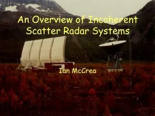
Incoherent Scatter Radar as a tool for M-I coupling studies Ian McCrea Jackie Davies SSTD Rutherford Appleton Laboratory Chilton, Oxfordshire UK
Structure of this talk • Why study the magnetosphere with radars ? • What can IS radars do ? • What can’t they do ? • What other toys do we need ? • Cluster in particular • What did we start out to do ? • What have we actually done ? • What kind of science has come out ? • What do we still need to do ? • What’s next ? • THEMIS, MMS and Cross-Scale • AMISR and EISCAT-3D
Why study the magnetosphere from the ground ? • Converging field geometry projects very diverse regions to small areas: Ai ~ Am * (Bm/Bi) • Measure boundaries and boundary conditions (e.g. conductivities, heating rates) • Possibility for conjugate observations and time history of a field line • Resolution of spatial and temporal effects
Strengths of ISRs • Backscatter is continuous in range • Continuous time series allows study of dynamics • Steerability and flexible pulse-coding allow great freedom in experiment design • Multi-parameter data sheds light on various aspects of MI processes • Standard interpretation of features (OCB, PIFs etc) Moen et al, Ann. Geophys., 22, 1973, 2004
Weaknesses of ISRs • Limited by SNR, especially at long range • Assumptions may not always work (non-thermals, composition) • Limited viewing area, so lack of spatial context. • Velocity determination not good in far field • Ambiguity in moving events Lockwood et al, PSS, 36, 1229, 1988 Lockwood et al, Nature 361, 424, 1993
Weaknesses of ISRs • Limited by SNR, especially at long range • Assumptions may not always work (non-thermals, composition) • Limited viewing area, so lack of spatial context. • Velocity determination not good in far field • Ambiguity in moving events Lockwood et al, Nature 361, 424, 1993
Weaknesses of ISRs • Limited by SNR, especially at long range. • Assumptions may not always work (non-thermals, composition) • Limited viewing area, so lack of spatial context. • Velocity determination not good in far field • Ambiguity in moving events Lockwood et al, Nature 361, 424, 1993
ISR and SUPERDARN observations are different, but strongly complementary Both have their own strengths and weaknesses Davies et al, Ann. Geophys., 20, 781, 2002
More from the toolbox Combination of ISR and imager data shows correspondence of optical and radar features Assimilative electrodynamics from magnetometers etc, and combination with ISR data Carlson et al, GRL, 33, L05103, 2006 Lühr et al, Ann. Geophys, 14, 162, 1996
Cluster Science Topics • Magnetopause reconnection and Flux Transfer Events • Dynamics and structure of the cusp region • Wave-particle interaction in the cusp • Formation and properties of the LLBL • Large-scale waves at the flank magnetopause • Particle acceleration during magnetotail reconnection • Dynamics and properties of magnetotail current sheet • Physics of magnetospheric substorms • Structure of flux ropes in the magnetotail
ESR Cluster Experiments • Uses 32m dish and interleaved 42m (4:1) • 42m dish is fixed field-aligned (az 182o, el 81o) • Cusp conjunctions use 32m radar in LowElNorth mode (az 336o, el 30o) • Tail conjunctions often use 32m radar in LowElSouth mode (az 167.7o, el 30o) • Tau0 modulation alternating code 20 s baud • Basic range resolution 3.0 km (~30 km in F-region) • Basic time resolution 6.4s • Range coverage 119 To 1366 km • Mag. Latitude coverage 76o To 80o (Low El North) • Mag. Latitude coverage 74o To 67o (Low El South)
VHF Cluster Experiments • Radar pointed geographic north (azimuth 359.5o, 30o elevation) • Dual beam experiments initially • Tau1 modulation scheme • Alternating code experiment (baud 24s) • Basic range resolution 3.6 km (typically 20 km in F-region) • Altitude Coverage 77km to 1268 km • Mag. Latitude Coverage (67.7oN) 73oN to 80oN • Basic time resolution 5s (60s in analysis) • Standard analysis by GUISDAP
Cusp Sector:March 16 2006 • Footprints generally over Svalbard, or further North • Emphasis on latitudinal coverage, flow transients etc. • ESR continues latitude coverage north of VHF viewing area • ESR field-aligned data provide a second perspective on plasma passing over Svalbard
Cusp Sector:March 16 2006 • February to April each year • Emphasis on magnetopause crossings • Conjugacy with Tromsø/ESR • 4-hour experiments • Consistency with SUPERDARN • Hand-on to Sondy • >70 EISCAT/Cluster cusp experiments since 2001
Cusp Sector Modes: ESR Low El North, VHF Dual Beam CP4
Cusp Sector Modes: ESR Low El North, VHF Single Beam CP4
Cusp Sector Modes Tromsø Range coverage 151 to 2100 km Height coverage 77 to 1268 km Mag lat coverage (67) 73 – 80oN Geo lat coverage (73) 76 – 83oN ESR Range coverage 148 – 1295 km Height coverage 76 – 737 km Mag lat coverage 76o – 80o Geog lat coverage 79o – 84o L T
Multi-radar dataPoleward Moving Forms4 October 2002 K.A. McWilliams, University of Saskatchewan
Tail Conjunction Modes • Footprints generally between Svalbard and Tromsø • Emphasis on coverage of auroral region • VHF beam covers some latitudes north of ESR • ESR covers some latitudes sourth of VHF viewing area • ESR field-aligned data see e.g. plasma emerging from polar cap
Tail Conjunction Modes: ESR Low El South, VHF Dual Beam CP4
Tail Conjunction Modes: ESR Low El South, VHF Single Beam CP4
Tail Conjunction Modes Tromsø Range coverage 151 to 2100 km Height coverage 77 to 1268 km Mag lat coverage (67) 73o – 80o Geo lat coverage (73) 76o – 83o ESR Range coverage 148 – 1295 km Height coverage 76 – 737 km ESR mag lat coverage 74o-67o ESR geog lat coverage 77o-69o L T
Perigee Passes • Occur at all times of year • Generally 2-3 suitable passes a month • Frequently we do not cover these • Same mode as cusp sector passes • Should we do more ?
Flank Skimming/Flank Crossing Orbits • Occur in the summer and winter • Oriented for phenomena such as waves on the flanks • Same mode as cusp sector passes • Less frequent runs and less scientific interest in these months ?
Sondrestrom ISR 1300 MHz 3 MW 32 m dish
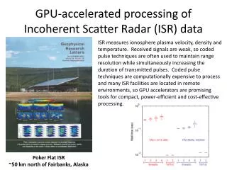
First Cluster Cusp Encounter • First Cluster pass through the ionospheric cusp • a) Magnetic field at ACE satellite orbiting upstream of the Earth at the Lagrange point • d) Energy of the particles observed by Cluster • b) and c) Ionosphere as seen by the radar in particular, strongly enhanced high density features (red) are clearly visible moving away from the radar
Polar Cap Patches under Bz SouthLockwood et al, Ann. Geophys., 19, 1589, 2001a • Cluster outbound from tail lobe to dusk sector mantle • ESR sees poleward-moving patches, repetition frequency ~ 10 minutes • DMSP sees dispersed ion and electron signatures • Patches also pass over Cluster • Good correlation of low energy precipitation at EISCAT and low-energy sheath electrons at Cluster • Suggests a mechanism more complex than time elapsed since reconnection for controlling soft particle flux
Reconnection under High Clock AngleLockwood et al, Ann. Geophys, 19, 1613, 2001b • IMF turns north at 0945 (1100 at ionosphere) • Remains generally north, with excursions to intermediate clock angle • Cluster moving outbound through magnetosheath, with transient excursions into LLBL and cusp • Excursions coincide with clock angle swings • Poleward-moving transients seen at these times by ESR • Could be FTEs - not classical signatures, due to position in interior cusp ?
Pulsed Reconnection in By dominated IMFWild et al, Ann. Geophys., 23, 2903 2005 • Combines in-situ observations of pulsed reconnection by Cluster and Double Star. • Pulsed flows directed poleward and dawnward • Flux tubes anchored at mid-latitude and close to sub-solar point • Reconnection not limited to high latitudes in By dominated IMF
Conjugate Reconnection at Multiple HeightsFarrugia et al, Ann Geophys, 22, 2891, 2004 • Cluster/FAST/Sondy/SUPERDARN • Transient reconnection signatures at three altitudes • Cluster goes from cusp to boundary layer during a pressure pulse • Flow bursts seen at Cluster interpreted as Alfven waves in reconnection events • FAST sees stepped cusp signatures correspond to flow bursts • Sondy sees flow bursts poleward of convection reversal boundary • OCB equatorward of CRB • Momentum transfer in downstream boundary layer ?
Electrodynamics of Auroral ArcsAikio et al, Ann. Geophys., 22, 4089, 2004 • Cluster in midnight sector at 4 RE • Pseudo-breakup onset occurs • Current sheets of equatorward arc widen and FAC doubles in < 2 mins • Density cavity forms in the downward current region of poleward arc • Pedersen current decreased, return current region forms a growing load for current circuit • Electrons carrying return current accelerated and region widens to supply required amount of return current • Evidence of Alfven wave acceleration of electrons in the upward FAC
Possible new sites Possible new baseline Transmitter site 69.4 N 30.0 E EISCAT-3D • A common transmitter facility with RX capabilities: • Close to the present Tromsø (NO) EISCAT site • Operating frequency in the (225-240) MHz range • Power amplifiers utilising VHF TV power FETs • Phased-array system with > 16 K elements, Ppk > 2 MW • Actual antenna configuration and performance TBD • >3 outlier, RX-only array modules for interferometry • Fully digital, post-sampling beam-forming on receive • Comprehensive interferometric capabilities built-in • 2 + 2 very large receive-only (”remote”) arrays: • Actual siting TBD, four promising sites investigated... • Filled apertures, long enough to provide ~ 1 km beam resolution at E region altitudes above transmitter • Medium gain (~ 10 dBi) element antennas • Fully digital, post-sampling beam-forming • Sufficient local signal processing power to generate • at least five simultaneous beams • 10 Gb/s connections for data transfer and remote • control and monitoring 69.58 N 19.22 E 68.2 N 14.3 E ~67 N Present idea of the EISCAT 3D system geometry. The central core (denoted by a green filled circle) is assumed to be located near the present Norwegian EISCAT site at Ramfjordmoen. The dashed circle with a radius of approximately 250 km indicates the approximate extent of the central core FOW at 300 km altitude. Receiving sites located near Porjus (Sweden) and Kaamanen (Finland) provide 3D coverage over the (250-800) km height range, while two additional sites near Abisko (Sweden) and Masi (Norway) cover the (70-300) km height range.
The EISCAT_3D Test Array (“Demonstrator”) • 200 m2 filled array now being erected at EISCAT Kiruna site to provide facilities for validating several critical aspects of a full-scale 3D receiving array in practice under realistic climatic conditions: • Receiver front ends, A/D conversion (WP 4), • SERDES, copper/optical/copper conversion (WP 12), • Time-delay beam-steering (WP4 / WP9), • Simultaneous forming of multiple beams (WP 9), • Adaptive pointing (self-) calibration (WP 9), • Adaptive polarisation matching (WP 9), • Interferometry trigger processor (WP 5), • Digital back-end / correlator for standard IS (WP 9), • Time-keeping (WP12) • Array oriented in Tro-Kir plane; 48 short (6+6) element Yagis at 55oelevation, • Center frequency of (224 ± 3) MHz allows reception of transmissions from existing Tromsø VHF system.SNR estimated to be sufficient for useful bistatic IS work (> 6% @ 300 km, 1.0 1011 m-3), • The 55oelevation provides coverage from ~ 200 km altitude to over 800 km above Tromsø. D cos D sin • D selected to make ( D sin ) optimal stacking distance BEAM DIRECTION N D R1 R4 R12
Conclusion • CGBWG is helping to assemble a unique set of radar data for MI coupling studies (credit to Jim Wild, Gareth Chisham, Steve Milan and many others) • Huge thanks are due to the staff at EISCAT and Sondy ! • All ISR data are on-line via Madrigal • http://www.openmadrigal.org/ • Cluster Ground-Based Working Group • http://www.ion.le.ac.uk/~cluster • Feedback needed: • What else should the ISRs be doing ? • Are these the right modes ? • What modes are needed to support new missions ?