Download
1 / 14
140 likes | 376 Vues
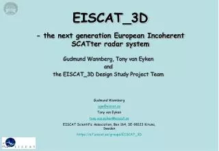
EISCAT_3D - the next generation European Incoherent SCATter radar system. Gudmund Wannberg, Tony van Eyken and the EISCAT_3D Design Study Project Team. Gudmund Wannberg ugw@eiscat.se Tony van Eyken tony.van.eyken@eiscat.se EISCAT Scientific Association, Box 164, SE-98123 Kiruna, Sweden

E N D
EISCAT_3D- the next generation European Incoherent SCATter radar system Gudmund Wannberg, Tony van Eyken and the EISCAT_3D Design Study Project Team Gudmund Wannberg ugw@eiscat.se Tony van Eyken tony.van.eyken@eiscat.se EISCAT Scientific Association, Box 164, SE-98123 Kiruna, Sweden https://e7.eiscat.se/groups/EISCAT_3D
How the European Union came to support the next generation EISCAT system: Many elements of a case for the post-2006 EISCAT in place by early 2003: • National White Papers by Germany, Sweden, UK, • The E’ concept, • and input from individuals: • Improved middle atmosphere and topside performance, • 5 – 10 times better temporal and spatial resolution, • interferometric capabilities, etc. • But a shortage of resources… 2003: The EU 6th Framework Programme“Structuring the European Research Arena” • 6th Framework Programme established to support the creation of new science networks based on existing infrastructure, • Sub-Programme for Design Studies for new science infrastructure, • Application for support for the EISCAT_3D Design Study submitted to Brussels on September 30, 2004, • Application evaluated favourably ! • Contract negotiations between EU and EISCAT and other Parties successfully concluded in March, 2005: • Four-year project • EU FP6 contribution not more than 2,017,445 EUR (~ 2.6 M USD) • An equivalent amount to be contributed by the Parties (i.e. EISCAT and partners) • EISCAT to invest a total of 126 man-months of effort over 4 yrs, corresponding to ~ 2.7 full-time positions on average • 3D Design Study formally started on May 1, 2005 Topics to be addressed by the Design Study: • Establishing users’ requirements in more detail • Baseline Specification • Frequency allocations / protection • Options for RF power generation, TX antenna • Siting options, RF environment, logistics, ... • RX performance criteria: • dynamic range, NF, bandwidth, ... • Prototype RX (224 MHz RF -> serial bit stream) on silicon • Communications protocols, digital beam-forming and signal pre-processing • Data storage/archiving/dissemination • Verification of real-time multibeaming w/ simultaneous pointing auto-calibration on small demonstrator array • Preliminary costing If everything goes well, a 3D system may be on the air by 2012-2013
The 3D Study is sub-divided into Work Packages: • WP1 Management / Spectrum EI • WP2 Evaluation of design performance goals ALL • WP3 Active element (transmitter) options EI, UIT • WP4 Phased array receiver design LTU, EI • WP5 Interferometry UIT, EI • WP6 Active element design EI • WP7 Distributed control and monitoring EI • WP8 Data archiving and distribution RAL, EI • WP9 Signal processing EI, UIT • WP10 New developments UIT • WP11 Implementation blueprint EI • WP12 Time and frequency EI • WPs 1, 3, 4, 5, 7, 8, 9, 10 and 12 currently running. • WP 2 completed in November 2005 • Baseline Specification Legend: EI = EISCAT UIT= Univ. of Tromsø (NO) LTU= Luleå Univ. of Technology (SE) RAL= Rutherford Appleton Laboratories (UK) Project Timeline April 30, 2009
EISCAT_3D Design targets and Central Core Layout Central core parameters: First phase Fully instrumented Number of elements: 16 K 30 K Diameter [wavelengths]: 87 116 Element separation [wl]: 0.6 0.6 P x A [GW m-2]: 91 295 Half Power BW [degrees]: 0.62 0.46 Cf. the EISCAT VHF system in Mode 1 (full antenna, 3 MW): P x A = 2.4 GW m-2, HPBW = 0.6 x 1.7 degrees
Possible new sites Possible new baseline Transmitter site 69.4 N 30.0 E Present idea of 3D TX/RX configuration • A common transmitter facility with RX capabilities: • Close to the present Tromsø (NO) EISCAT site • Operating frequency in the (225-240) MHz range • Power amplifiers utilising VHF TV power FETs • Phased-array system with > 16 K elements, Ppk > 2 MW • Actual antenna configuration and performance TBD • >3 outlier, RX-only array modules for interferometry • Fully digital, post-sampling beam-forming on receive • Comprehensive interferometric capabilities built-in • 2 + 2 very large receive-only (”remote”) arrays: • Actual siting TBD, four promising sites investigated... • Filled apertures, long enough to provide ~ 1 km beam resolution at E region altitudes above transmitter • Medium gain (~ 10 dBi) element antennas • Fully digital, post-sampling beam-forming • Sufficient local signal processing power to generate • at least five simultaneous beams • 10 Gb/s connections for data transfer and remote • control and monitoring 69.58 N 19.22 E 68.2 N 14.3 E ~67 N Present idea of the EISCAT 3D system geometry. The central core (denoted by a green filled circle) is assumed to be located near the present Norwegian EISCAT site at Ramfjordmoen. The dashed circle with a radius of approximately 250 km indicates the approximate extent of the central core FOW at 300 km altitude. Receiving sites located near Porjus (Sweden) and Kaamanen (Finland) provide 3D coverage over the (250-800) km height range, while two additional sites near Abisko (Sweden) and Masi (Norway) cover the (70-300) km height range.
3D Interferometry requirements – consequences for the core array design(data courtesy of Tom Grydeland/Cesar la Hoz, UiT) To form the longest baselines, 3 or more outlier, RX-only modules will be deployed at up to 1500 m from the array midpoint. The main aperture diameter should be at least 150 (188 m) to enable these baselines to be constructed internal to the aperture. This accommodates 25 or more 6- modules and matches the aperture size required for target IS performance very well indeed ! This suggests that the main array should be organised hierarchically, with elements grouped together in small groups of diameter 6 (7.5 m).
EISCAT_3D Receiver Front End Assumptions: • The receiver front end is a key element in the 3D project: • Digital beam-steering and multi-beaming requires that the data from every element antenna is available in digital format, i.e. every antenna must have an ADC fitted, • To reduce the front-end component count, straight amplification followed by constructive under-sampling will be employed (sampling clock running at ~ 80 MHz, signal at ~ 235 MHz in 6th Nyqvist zone), • Large bandwidth (> 15 %) low-noise performance at VHF requires unusual design choices in first amplifier stage (X band medium power GaAsFET…) • Because of the presence of the remote sites, the total number of receivers is more than twice the number of active elements (> 30000) ; therefore a common front end design will be developed and used throughout the system, • It is planned to eventually develop fully integrated front end systems on silicon, • This slide illustrates the proof-of-concept work currently going on in connection with the Demonstrator array; a total of 24 front ends of this design to be built. • Bipolar 2s complement ADC with full-scale voltage = ± 0.5 volt • 12 bits (b0 – b11) • 50+j0 ohm input impedance • Noise floor established by amplified sky/antenna/preamp noise • Gaussian white noise • RMS noise voltage, UN at the 3-bit level • Very low SNR • Equivalent noise BW = 10 MHz Quick-and-dirty estimate of required front-end gain: • Voltage per ADC bit: • Ub(i) = 0.5 • 2(i -10) • Set the front-end power gain G such that |UN| equals b2: • UN = (G • (4 k T B RL))0.5= 0.5 • 2(2-10) = 1.953 exp (- 3) V • Known quantities: • k = 1.38 10-23 • T = 150 K • B = 107 Hz • RL = 50 ohm Block diagram of Demonstrator front end ADC_CLK 80 MHz RF 235 MHz A 1 A 2 A 3 ADC 12b, 80 Ms/s | 4 k T B RL | = 1.035 exp (-12); A 1: MGF1801 G = 21 dB, Tn = 25 K A 2, A3: MGA62563 G = 23 dB, Tn = 60 K FL1: BPF G = -2 dB, BW = 10 - 30 MHz G = UN2 / | 4 k T B RL | = 65.7 dB Gtot = 65 dB, Tn, tot = 26 K
Digital time-delay beam-steering • Time-delay beam-steering (TDS) will be used throughout, as opposed to phase steering, for the following reasons: • The 3D system will be employing large BW modulations (up to 5 MHz), • Plasma line reception at frequency offsets of up to 15 MHz (7% of the center frequency) at large off-boresight angles will be a routine feature, in particular at the remote sites, • But phase steering modulo-2 is dispersive, i.e. the beam direction is a function of the frequency offset, so won’t work in our case ! • OTOH, TDS is non-dispersive and will maintain the beam direction irrespective of frequency offset ! • The solution: • Better than 10 ps time resolution can be achieved by inserting so-called fractional sample delay (FSD) filters in the signal paths. • The basic FSD technique has been discussed in the literature in the context of e.g. multi-beaming phased-array sonar systems (1,2) and is also beginning to show up in radio astronomy applications. It is based on the fact that a band-limited signal cannot contain components with infinite rates of change of phase or amplitude. If a band-limited signal is sampled for a sufficiently long time, the sample series can be interpolated to find the signal value at any intermediate time, down to an arbitrary fraction of a sample interval. In practice, the interpolation is realised in an all-pass digital FIR filter, whose coefficients are selected to produce the required delay at the output. • Extensive Matlab simulations have shown that 48-tap FIR filters can be designed to provide almost constant group delay across the full 3D receiving bandwidth (30 MHz), albeit with some residual amplitude ripple in the passband; the FSD technique really does work with _3D parameters ! • The problem: • When implementing the TDS system for the 3D radar, we must find a reliable way to resolve time down to the sub-nanosecond level: • The target value for the beam pointing resolution is 0.625o in each of two orthogonal planes. • This requires that the element-to-element delay be settable to a resolution of 0.018 · (1/2) ns = 12.7 picoseconds! • BUT- the sampling will be running at about 80 MHz / 12.5 ns per sample (103 times longer!); how to reconcile ? References: 1. Murphy, N.P., A. Krukowski and I. Kale, Implementation of a Wide-Band Integer and Fractional Delay Element, Electronics Letters, 30, No. 20, pp. 1658-1659 (1994) 2. Murphy, N.P., A. Krukowski and A. Tarczynski, An Efficient Fractional Sample Delayer for Digital Beam Steering, Proceedings of ICASSP ’97 (1997)
Digital beam-forming: beam-forming logic, multi-beaming and beam errors A digital beam-former (BF) consists of two main parts, viz. a set of fractional sample delay (FSD) units and a full- adder (). BF 16 s0 s-1 s-2 s-3 s-n c-1 c-2 c-3 c-n X X X X FSD One FSD unit is required per element antenna and beam. It can be realised as a generic FIR filter structure in FPGA logic. The coefficients c-m, m= 1…n, determine the filter group delay and must be computed for each element antenna and beam direction. ADC timing jitter and other timing errors affect the beam, but when the error distribution is Gaussian, the average pointing direction stays the same regardless of the width of the distribution. On the other hand, Gaussian timing jitter causes a widening of the beam and a loss of gain. A 3- jitter of 100 ps results in a 0.1 dB gain loss; 500 ps jitter results in almost 2 dB gain loss ! Clock distribution and ADC sampling stabilisation now become important issues; in order not to lose performance, the system must be designed for a 3- jitter of less than 100 ps, array-wide. U-1 Summing the delayed outputs from all FIR filters in the full-adder generates the beam-formed data stream. Beam-formed data Multiple beams can be generated from the same data by simply adding more beam-formers, one per beam!
Current view of EISCAT_3D central core data flow and signal processing • Front ends: • 16 bit sampling • 80 MHz sample rate • 2 polarisation streams/element • 1.28 Gb/s per polarisation • 2.56 Gb/s per element • Array subdivided into modules: • 24 x 24 elements/module • 32 modules (tentatively) • 18876 elements per array • Array data rate 47.19 Tb/s • = 5.90 TB/s !!! • ~ 17s on a 100 TB buffer • Storing data at this rate is obviously out of the question, the data rate must first be brought down to something in the order of the element data rate…
EISCAT_3D data types and data storage: Beam-formed data After beam-forming, each data stream represents the sum of delayed signals from all nel array elements (nel = 18876 in the present case), thus bringing the data rate back to the element rate of 1.28 Gb/s/polarisation. These are complex-amplitude data. Cannot be integrated, but could be decimated to reduce the data rate when deemed acceptable. H, V polarisations kept separate. Data rate/beam 2.56 Gb/s (1152 GB/H 27.6 TB/day, 10 PB/year). Storing full bandwidth beam-formed data is still very difficult/expensive, The standard procedure will therefore be to buffer beam-formed data for a limited time, allowing users to down-load interesting intervals to their own storage. • A possible COTS-based solution to the ring buffer problem: • Conduant MarkVa/MarkVb VLBI Data Recorder • developed by the VLBI group at Haystack, in conjunction with a commercial firm (Conduant) that sells these systems commercially: http://www.conduant.com/products/mark5vlbi.html • 19" rack mounted unit, comprising a PC with 2 "diskpacks“ each containing 8 off-the-shelf hard drives. Each diskpack is 3.2 TB with (very approx.) dimensions of 15x25x40cm • - The software will auto-swap the disk packs as they fill up. When not being used, the "other" disk pack may be hot-swapped, thus, with supervision, the MarkVa can sustain continuous operation. • - Each MarkVa can record at 1 Gbit/s. MarkVb 2 Gbit/s ! • - The EVN has been using MarkVa systems for about 1 year with no problems. • - Haystack provide VLBI technical support for the system, see http://web.haystack.mit.edu/mark5/ for details. Assuming a receiver duty factor of 80%, a MarkVb-compliant Conduant unit will cope with the data rate from a single beam and provide about six hours of ring buffer capacity!
More 3D Data Products: Analysed data Correlated data A representative analysed data set will always be generated and stored Each beam analysed separately Standard pre-integration Standard, well documented analysis procedure (GUISDAP), Well defined analysis strategy Long term storage (archive) Volumes about n times now (since n simultaneous beams) File-based data (easy to access particular dates/experiments) Relational tables (easier event identification and searching). The first “permanent” data product: Polarisations combined for max SNR, Sample matrix inflated into lag profiles, Time-windowing applied at remotes to match signal reception phase of each IPP, Time integration applied to further reduce data vector size, Data volumes manageable; e.g., 150 gates per profile @ 50 lags/gate generates about 150-200 MB/hour/beam. Interferometry data 10-15 baseline pairs used in coherence detection, Threshold logic monitors coherence levels and signals the storage system when predefined thresholds are exceeded, Beam-formed data from each array module used as an interferometer baseline endpoint (decimated to ion line BW) are then written to short-term (ring-buffer) storage, Interferometry users are automatically alerted and asked to copy the data to their own storage. Most data products available in near-real time via the Web!
The EISCAT_3D Test Array (“Demonstrator”) • 200 m2 filled array now being erected at EISCAT Kiruna site to provide facilities for validating several critical aspects of a full-scale 3D receiving array in practice under realistic climatic conditions: • Receiver front ends, A/D conversion (WP 4), • SERDES, copper/optical/copper conversion (WP 12), • Time-delay beam-steering (WP4 / WP9), • Simultaneous forming of multiple beams (WP 9), • Adaptive pointing (self-) calibration (WP 9), • Adaptive polarisation matching (WP 9), • Interferometry trigger processor (WP 5), • Digital back-end / correlator for standard IS (WP 9), • Time-keeping (WP12) • Array oriented in Tro-Kir plane; 48 short (6+6) element Yagis at 55oelevation, • Center frequency of (224 ± 3) MHz allows reception of transmissions from existing Tromsø VHF system.SNR estimated to be sufficient for useful bistatic IS work (> 6% @ 300 km, 1.0 1011 m-3), • The 55oelevation provides coverage from ~ 200 km altitude to over 800 km above Tromsø. D cos D sin • D selected to make ( D sin ) optimal stacking distance BEAM DIRECTION N D R1 R4 R12
Demonstrator element antennas Two short, 224-6RM (6+6) element X yagi antennas for (224 ± 3) MHz have been purchased from M2 Inc. Fresno, CA for evaluation. Another 46 are on order… E plane pattern Gain and VSWR vs. frequency The first two element antennas assembled and installed H plane pattern E plane pattern (four antennas, stacked broadside)