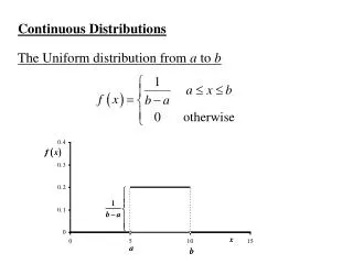
Validity and Applications of Continuous Distributions in Statistical Analysis
610 likes | 734 Vues
This document explores the validity and applications of continuous distributions, with a focus on the normal distribution, also known as the Gaussian distribution. The historical context of its discovery by Abraham de Moivre and Karl Friedrich Gauss is provided, alongside its properties and significance in statistical methods. The implications for biological data, such as blood pressure and height, are discussed. The paper also details methods for assessing whether data follow a normal distribution through graphical techniques and goodness-of-fit tests, emphasizing the practical applications in medical statistics.

Validity and Applications of Continuous Distributions in Statistical Analysis
E N D
Presentation Transcript
Validity and application of some continuous distributions Dr. Md. Monsur Rahman Professor Department of Statistics University of Rajshahi Rajshshi – 6205 E-mail: monsur_st_ru@yahoo.com
Normal distribution The first discoverer of the normal probability function was Abraham De Moivre(1667-1754), who, in 1733, derived the distribution as the limiting form of the binomial distribution. But the same formula was derived by Karl Freidrich Gauss(1777-1855) in connection with his work in evaluating errors of observation in astronomy. This is why the normal probability is often referred to as Gaussian distribution.
X: Normal Variate Density: Standard Normal Variate :
Properties of Normal distribution Normal probability curve is symmetrical about the ordinate at Mean, median and mode of the distribution are equal and each of these is The curve has its points of inflection at By a point of infection, we mean a point at which the concavity changes All odd order moments of the distribution about the mean vanish The values of and are 0 and 3 respectively
includes about 68.27% of the population includes about 95.45% of the population includes about 99.73% of the population Application: Many biological characteristics conform to a Normal distribution - for example, heights of adult men and women, blood pressures in a healthy population, RBS levels in blood etc.
Validity of NormalDistribution for a set of data Many statistical methods can only be used if the observations follow a Normal Distribution. There are several ways of investing whether observations follow a Normal distribution. With a large sample we can inspect a histogram to see whether it looks like a Normal distribution curve. This does not work well with a small sample, and a more reliable method is the normal plot which is described below.
X: Normal Variate Density: Standard Normal Variate :
CDF OF X : F(X) CDF OF Z : , P quantile of X : P quantile of Z : is the solution of is the solution of
Dataset • Find empirical CDF values • Arrange the data in ascending order as • Empirical CDF values are as follows • Using normal table obtain the values • corresponding to
If the given set of observations follow normal distribution, the plot (x, z) should roughly be a straight • line and the line passes through the • point and has slope . • Graphical estimates of and may be obtained. • If the data are not come from Normal distribution we • will get a curve of some sort.
Table 1 : RBS levels(mmol/L) measured in the blood of 20 medical students. Data of Bland(1995), pp. 66 2.2 3.6 3.8 4.1 4.7 3.3 3.6 3.8 4.1 4.7 3.3 3.7 3.9 4.2 4.8 3.4 3.8 4.0 4.4 5.0 Bland,M.(1995): An Introductions to Medical Statistics, second edition, ELBS with Oxford University Press.
Goodness of Fit Test • We use here Kolmogorov-Smirnov (KS) test • for the given data • KS statistic=max |CDF_FIT- CDF_EMP| • For the RBS level data we calculate KS statistic • KS(cal)=0.07827 • 5% tabulated value=0.294 • Conclusion: Normal distribution fit is good for the • given data
Results • Estimated population having RBS within the normal • range (3.9 – 7.8mmol/L) is about 51% • Estimated population having RBS below the normal • range is about 49% • Estimated population having RBS above the normal • range is 0%
Two sample case • Empirical CDF values of are • as follows: • Obtain the values corresponding to • Similarly values are obtained corresponding to
If the first set of data come from normal distribution • with mean and variance , then the plot • will roughly be linear and passes • through the point with slope . • If the second set of data come from normal distribution • with mean and variance , then the plot • will roughly be linear and passes • through the point with slope .
Both the lines parallel indicating different means • but equal variances • Both the lines coincide indicating equal means and • equal variances • Both the lines pass through the same point on the • X-axis indicating same means but different • variances
Table 2 : Burning times (rounded to the nearest tenth of a minute) of two kinds of emergency flares. Data due to Freund and Walpole(1987), pp. 530 Freund, J.E. and Walpole, R.E.(1987): Mathematical Statistics, Fourth edition, Prentice-Hall Inc.
Above plot indicates that both the samples come from normal population with unequal means and variances
Log-normal distribution In probability theory, a log-normal distribution is a probability distribution of a random variable whose logarithm is normally distributed. If X is a random variable with a normal distribution, then Y = exp(X) has a log-normal distribution; likewise, if Y is log-normally distributed, then X = log(Y) is normally distributed. It is occasionally referred to as the Galton distribution.
Density: Mean = Variance= Median= Mode=
Log-normal density function f(x) x
Application Certain physiological measurements, such as blood pressure of adult humans (after separation on male/female subpopulations), vitamin D level in blood etc. follow lognormal distribution. Subsequently, reference ranges for measurements in healthy individuals are more accurately estimated by assuming a log-normal distribution than by assuming a symmetric distribution about the mean.
Table 3 : Vitamin D levels(ng/ml) measured in the blood of 26 healthy men. Data due to Bland(1995), pp. 113 Bland,M.(1995): An Introductions to Medical Statistics, Second edition, ELBS with Oxford University Press.
MLE ng/ml ng/ml
Goodness-of-fit test • KS statistic=max |CDF_FIT- CDF_EMP| • For the vitamin D level data we calculate KS statistic • KS(cal)=0.0967 • 5% tabulated value=0.274 • Conclusion: Lognormal distribution fit is good for the • given vitamin D data
Results • Estimated population having vitamin D level within • the normal range (30 – 74 ng/ml) is about 56% • Estimated population having vitamin D level below • the normal range is about 40% • Estimated population having vitamin D level above • the normal range is about 4%
Weibull Distribution Weibull distribution is used to analyze the lifetime data • T: Lifetime variable • Density function • :Scale parameter(.632 quantile) • :Shape parameter(<1 or >1 or =1) • CDF : • Reliability (or Survival) function:
Hazard Function : • Increasing hazard rate : for • Decreasing hazard rate: for • Constant hazard rate : for p quantile, which is the solution of • Accordingly,
Exponential distribution • Weibull distribution reduces to exponential distribution • when Density function: • : Scale parameter(.632 quantile) • CDF : • Reliability (or Survival) function:
Hazard Function : p quantile, which is the solution of • Accordingly,
The red curve is the exponential density The red line is the exp. hazard function
Validity of Weibull distribution for a set of data From the Weibull CDF we get where • Ordered lifetimes are: • values are obtained through the empirical CDF values as given below
If the data follow Weibull distribution with scale • parameter and shape parameter , • the plot of (X,Y) will roughly be linear with slope • and passes through the point . • Accordingly, the graphical estimates of • and may be obtained.
Table 4: Specimens lives (in hours) of a electrical insulation at temperature appear below. Data due to Nelson(1990), pp. 154 Nelson,W.(1990): Accelerated Testing: Statistical Models, Test Plans, and Data Analyses, John Wiley and Sons.
MLE of and • Log-likelihood function of and based • on observed data • MLE of and by maximizing the • log-Likelihood with respect to and • using numerical method. • Graphical estimates may be used as starting • values required for the numerical method • The MLEs of and are denoted by • and respectively.
For the insulation fluid data given in table 4 the following results (based on MLEs) are obtained: hours hours Estimated median life= 3099.548 hours • ML estimate of R(t) Time (hour): 3000 3500 3700 4000 Reliability : .6124 .0807 .0107 .0000311
Weibull versus Exponential Model • Suppose we want to test whether we accept • exponential or Weibull model for a given set of • data • The above test is equivalent to test whether the • shape parameter of Weibull distribution is unity • or not i.e. vs
Test Procedure(LR test) • Under the log-likelihood function is • which yields , MLE of . • Maximum of is given by
Similarly, under the maximum of the • log-likelihood is given by where and are the MLE s of and under . • LR test implies follows chi-square • distribution with 1 df. • If , accept (use) • exponential Model
If , accept (use) Weibull • model • For the insulation fluid data given in table 4 Conclusion:Weibull model may be accepted at 5% level of significance
Stress: Temperature, Voltage, Load, etc. • Under operating (used) stress level, it takes • a lot of time to get sufficient number of failures • Lifetimes obtained under high stress levels • Aim: (i) To estimate the lifetime distribution • under used stress level, say, • (ii) To estimate reliability for a specified • time under • (iii) To estimate quantiles under Accelerated Life Testing (ALT) for Weibull Distribution
Sampling scheme(under constant stress testing) • Divide n components into k groups with number of components respectively, where • components exposed under stress levels • , j-th lifetime corresponding to • Obtain the equation for the lifetime corresponding to i-th group