Plotting the charge density of bulk Si

1. Plotting the charge density of bulk Si

2. Bulk Si: a covalent solid that crystallizes in the diamond structure The theoretical lattice constant of Si for this first example FCC lattice + a basis of two atoms Sampling in k in the first Brillouin zone to achieve self-consistency Go to the directory where the exercise on the structure of Si is stored Inspect the input file, Si.fdf More information at the Siesta web page http://www.icmab.es/siesta and follow the link Documentations, Manual Diamond structure:

3. Bulk Si: a covalent solid that crystallizes in the diamond structure Inspect the input file, Si.fdf Take a look to these input variables to produce the required files to plot charge densities More information at the Siesta web page http://www.icmab.es/siesta and follow the link Documentations, Manual

4. denchar plots the charge density and wave functions in real space atomic orbitals Coefficients of the eigenvector with eigenvalue density matrix Wave functions Charge density

5. denchar operates in two different modes: 2D and 3D 2D • Charge density and/or electronic wave functions are printed on a regular grid of points contained in a 2D plane specified by the user. • Used to plot contour maps by means of 2D graphics packages. 3D • Charge density and/or electronic wave functions are printed on a regular grid of points in 3D. • Results printed in Gaussian Cube format. • Can be visualized by means of standard programs (Moldel, Molekel, Xcrysden)

6. How to run denchar… siesta WriteDenchar .true. WriteWaveFunctions .true. %block WaveFuncKPoints 0.0 0.0 0.0 %endblockWaveFuncKPoints Only if you want to plot wave functions Output of siesta required by denchar SystemLabel.PLD SystemLabel.DIM SystemLabel.DM SystemLabel.selected.WFSX (only if wave functions) ChemicalSpecies.ion (one for each chemical species) denchar $ ln –s ~/siesta/Src/denchar . $ denchar < dencharinput.fdf You do not need to rerun siesta to run denchar as many times as you want

7. How to compile denchar… Go to the directory with the package $cd Util/Denchar/Src And type $make OBJDIR=Obj/ Where OBJDIR should point to the directory where the arch.make you want to use is located

8. Input of denchar General issues • Written in fdf (Flexible Data Format), as in siesta • It shares some input variables with siesta • SystemLabel • NumberOfSpecies • ChemicalSpeciesLabel • Some other input variables are specific of denchar (all of them start with “Denchar.”) • To specify the mode of usage • To define the plane or 3D grid where the charge/wave functions are plotted • To specify the units of the input/output • Input of denchar can be attached at the end of the input file of siesta

9. Input of denchar How to specify the mode of run Either one or the other (or both of them) must be .true. • Denchar.TypeOfRun (string) 2D or 3D • Denchar.PlotCharge (logical) .TRUE. or .FALSE. • If .true. SystemLabel.DM must be present • Denchar.PlotWaveFunctions (logical) .TRUE. or .FALSE. • If .true. SystemLabel.WFSX must be present

10. Input of denchar How to specify the plane Plane of the plot in 2D mode x-y plane in 3D mode • Denchar.PlaneGeneration (string) • NormalVector • TwoLines • ThreePoints • ThreeAtomicIndices • + more variables to define the • generation object (the normal vector, lines, points or atoms) • origin of the plane • x-axis • size of the plane • number of points in the grid • Different variables described in the User Guide (take a look to the Examples)

11. Input of denchar

12. Chosen plane in the example

13. To produce the figures of the densities and wave functions in real space $ siesta < Si.fdf > Si.out The selected wave functions are written in a file called Si.selected.WFSX and the files required to run DENCHAR are Si.PLD Si.DIM Si.DM ChemicalSpecies.ion (one for each chemical species) To run denchar and produce the corresponding output files for the wavefunctions, we have to rename the SystemLabel.selected.WFSX to SystemLabel.WFSX $ cp Si.selected.WFSX Si.WFSX rundenchar $ denchar < Si.fdf

14. Output of denchar 2D mode Wave functions Wave function for different bands (each wavefunction in a different file) .CON.K#.WF#.REAL .CON.K#.WF#.IMAG .CON.K#.WF#.MOD .CON.K#.WF#.PHASE where # after K is the number of k-point in the list, and # after the WF is the number of wavefunction for that k-point (in order of energy). The suffix (REAL, IMAG, MOD, PHASE) is self-explanatory (If spin polarized, suffix .UP or .DOWN) Charge density Spin unpolarized: self-consistent charge (.CON.SCF) deformation charge (.CON.DEL) Spin polarized: density spin up (.CON.UP) density spin down (.CON.DOWN) deformation charge (.CON.DEL) magnetization (.CON.MAG) Format

15. Output of DENCHAR 3D mode Charge density Wave functions Spin unpolarized: self-consistent charge (.RHO.cube) deformation charge (.DRHO.cube) Spin polarized: density spin up (.RHO.UP.cube) density spin down (.RHO.DOWN.cube) deformation charge (.DRHO.cube) Wave function for different bands (each wavefunction in a different file) same format as before but with the suffix .cube Format Gaussian Cube format Atomic coordinates and grid points in the reference frame given in the input Reference frame orthogonal

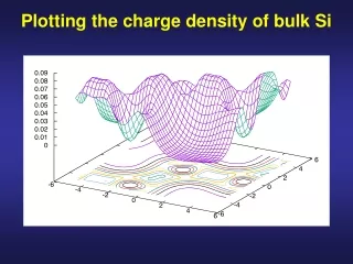
16. Visualization of the charge density If you have python with the libraries numpy and gnuplot installed $ surf.py Si.CON.SCF $ 2dplot.py Si.CON.SCF Replace the name of the file for one of your choice If not, you can edit the file surf.gplot $ vi surf.gplot set parametric set style data lines set hidden set contour base set cntrparam levels auto 10 splot "Si.CON.SCF" using 1:2:3 with lines notitle change the name of the file you want to plot in the last line, save the file and run: $ gnuplot surf.gplot

17. Visualization of the charge density