Download
1 / 69
710 likes | 1.07k Vues
Figure 9.1 Flow graph of 1 st -order complex recursive computation of X [ k ]. Figure 9.2 Flow graph of 2 nd -order recursive computation of X [ k ] (Goertzel algorithm). Figure 9.3 Illustration of the basic principle of decimation-in-time.

E N D
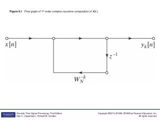
Figure 9.1 Flow graph of 1st-order complex recursive computation of X[k ].
Figure 9.2 Flow graph of 2nd-order recursive computation of X[k ] (Goertzel algorithm).
Figure 9.3 Illustration of the basic principle of decimation-in-time.
Figure 9.4 Flow graph of the decimation-in-time decomposition of an N-point DFT computation into two (N/2)-point DFT computations (N = 8).
Figure 9.5 Flow graph of the decimation-in-time decomposition of an (N/2)-point DFT computation into two (N/4)-point DFT computations (N = 8).
Figure 9.6 Result of substituting the structure of Figure 9.5 into Figure 9.4.
Figure 9.8 Flow graph of basic butterfly computation in Figure 9.9.
Figure 9.9 Flow graph of complete decimation-in-time decomposition of an 8-point DFT computation.
Figure 9.10 Flow graph of simplified butterfly computation requiring only one complex multiplication.
Figure 9.11 Flow graph of 8-point DFT using the butterfly computation of Figure 9.10.
Figure 9.15 Rearrangement of Figure 9.11 with input in normal order and output in bit-reversed order.
Figure 9.16 Rearrangement of Figure 9.11 with both input and output in normal order.
Figure 9.17 Rearrangement of Figure 9.11 having the same geometry for each stage, thereby simplifying data access.
Figure 9.18 Illustration of the basic principle of decimation-in-frequency.
Figure 9.19 Flow graph of decimation-in-frequency decomposition of an N-point DFT computation into two (N/2)-point DFT computations (N = 8).
Figure 9.20 Flow graph of decimation-in-frequency decomposition of an 8-point DFT into four 2-point DFT computations.
Figure 9.21 Flow graph of a typical 2-point DFT as required in the last stage of decimation-in-frequency decomposition.
Figure 9.22 Flow graph of complete decimation-in-frequency decomposition of an 8-point DFT computation.
Figure 9.23 Flow graph of a typical butterfly computation required in Figure 9.22.
Figure 9.24 Flow graph of a decimation-in-frequency DFT algorithm obtained from Figure 9.22. Input in bit-reversed order and output in normal order. (Transpose of Figure 9.15.)
Figure 9.25 Rearrangement of Figure 9.22 having the same geometry for each stage, thereby simplifying data access. (Transpose of Figure 9.17.)
Figure 9.26 Number of floating-point operations as a function of N for MATLAB fft ( ) function (revision 5.2).
Figure 9.27 Frequency samples for chirp transform algorithm.
Figure 9.29 An illustration of the sequences used in the chirp transform algorithm. Note that the actual sequences involved are complex valued. (a) g[n] = x[n]e−jω0n Wn2/2. (b) W−n2/2. (c) g[n] ∗W−n2/2.
Figure 9.30 An illustration of the region of support for the FIR chirp filter. Note that the actual values of h[n] as given by Eq. (9.48) are complex.
Figure 9.31 Block diagram of chirp transform system for finite-length impulse response.
Figure 9.32 Block diagram of chirp transform system for causal finite-length impulse response.
Figure 9.33 Block diagram of chirp transform system for obtaining DFT samples.
Figure 9.34 Flow graph for decimation-in-time FFT algorithm.
Figure 9.36 Linear-noise model for fixed-point round-off noise in a decimation-in-time butterfly computation.
Figure 9.37 (a) Butterflies that affect X[0]; (b) butterflies that affect X[2].
Figure 9.38 Butterfly showing scaling multipliers and associated fixed-point round-off noise.