Advanced Gene Recognition Techniques: GENCAN, EasyGene, Twinscan, and More
This presentation delves into advanced methodologies for gene recognition, detailing tools such as GENCAN, EasyGene, and Twinscan. It explores the intricacies of gene structure, including exons, introns, and coding potential, alongside crucial concepts like splicing, transcription, and translation. Additionally, it discusses approaches to gene finding, including homology-based methods and hidden Markov models. Emphasis is placed on splice site detection and the correlation between C+G content and gene parameters, highlighting the effectiveness of GENCAN in gene prediction accuracy.

Advanced Gene Recognition Techniques: GENCAN, EasyGene, Twinscan, and More
E N D
Presentation Transcript
Gene Recognition Credits for slides: Marina Alexandersson Lior Pachter Serge Saxonov
Reading • GENSCAN • EasyGene • SLAM • Twinscan Optional: Chris Burge’s Thesis
DNA transcription RNA translation Protein Gene expression CCTGAGCCAACTATTGATGAA CCUGAGCCAACUAUUGAUGAA PEPTIDE
Gene structure intron1 intron2 exon2 exon3 exon1 transcription splicing translation exon = coding intron = non-coding
Exon 3 Exon 1 Exon 2 Intron 1 Intron 2 5’ 3’ Stop codon TAG/TGA/TAA Start codon ATG Finding genes Splice sites
Approaches to gene finding • Homology • BLAST, Procrustes. • Ab initio • Genscan, Genie, GeneID. • Hybrids • GenomeScan, GenieEST, Twinscan, SGP, ROSETTA, CEM, TBLASTX, SLAM.
T A A T A T G T C C A C G G G T A T T G A G C A T T G T A C A C G G G G T A T T G A G C A T G T A A T G A A Exon1 Exon2 Exon3 GHMM for gene finding This is a HMM similar to the GENSCAN HMM duration
Elements of the HMM • Duration of states – length distributions of • Exons • Introns • Signals at state transitions • ATG • Stop Codon TAG/TGA/TAA • Exon/Intron and Intron/Exon Splice Sites • Emissions • Coding potential and frame at exons • Intron emissions
Better way to do it: negative binomial • EasyGene: Prokaryotic gene-finder Larsen TS, Krogh A • Negative binomial with n = 3
2. Splice Site Detection Donor: 7.9 bits Acceptor: 9.4 bits (Stephens & Schneider, 1996) (http://www-lmmb.ncifcrf.gov/~toms/sequencelogo.html)
Donor site 5’ 3’ Position % 2. Splice Site Detection
2. Splice Site Detection • WMM: weight matrix model = PSSM (Staden 1984) • WAM: weight array model = 1st order Markov (Zhang & Marr 1993) • MDD: maximal dependence decomposition (Burge & Karlin 1997) • Decision-tree algorithm to take pairwise dependencies into account • For each position I, calculate Si = ji2(Ci, Xj) • Choose i* such that Si* is maximal and partition into two subsets, until • No significant dependencies left, or • Not enough sequences in subset • Train separate WMM models for each subset G5G-1 G5G-1 A2 G5G-1 A2U6 G5 All donor splice sites not G5 G5 not G-1 G5G-1 not A2 G5G-1A2 not U6
atg caggtg ggtgag cagatg ggtgag cagttg ggtgag caggcc ggtgag tga
3. Coding potential Amino Acid SLC DNA codons Isoleucine I ATT, ATC, ATA Leucine L CTT, CTC, CTA, CTG, TTA, TTG Valine V GTT, GTC, GTA, GTG Phenylalanine F TTT, TTC Methionine M ATG Cysteine C TGT, TGC Alanine A GCT, GCC, GCA, GCG Glycine G GGT, GGC, GGA, GGG Proline P CCT, CCC, CCA, CCG Threonine T ACT, ACC, ACA, ACG Serine S TCT, TCC, TCA, TCG, AGT, AGC Tyrosine Y TAT, TAC Tryptophan W TGG Glutamine Q CAA, CAG Asparagine N AAT, AAC Histidine H CAT, CAC Glutamic acid E GAA, GAG Aspartic acid D GAT, GAC Lysine K AAA, AAG Arginine R CGT, CGC, CGA, CGG, AGA, AGG Stop codons Stop TAA, TAG, TGA
4. GENSCAN’s hidden weapon • C+G content is correlated with: • Gene content (+) • Mean exon length (+) • Mean intron length (–) • These quantities affect parameters of model • Solution • Train parameters of model in four different C+G content ranges!
Results of GENSCAN • On the initial test dataset (Burset & Guigo) • 80% exact exon detection • 10% partial exons • 10% wrong exons • In general • Most accurate single sequence-based gene predictor • In practice it overpredicts human genes by ~2x
Comparison of 1196 orthologous genes(Makalowski et al., 1996) • Sequence identity between genes in human/mouse • exons: 84.6% • protein: 85.4% • introns: 35% • 5’ UTRs: 67% • 3’ UTRs: 69% • 27 proteins were 100% identical.
Human Mouse Human-mouse homology
50 . : . : . : . : . : 247 GGTGAGGTCGAGGACCCTGCA CGGAGCTGTATGGAGGGCA AGAGC |: || ||||: |||| --:|| ||| |::| |||---|||| 368 GAGTCGGGGGAGGGGGCTGCTGTTGGCTCTGGACAGCTTGCATTGAGAGG 100 . : . : . : . : . : 292 TTC CTACAGAAAAGTCCCAGCAAGGAGCCACACTTCACTG |||----------|| | |::| |: ||||::|:||:-|| ||:| | 418 TTCTGGCTACGCTCTCCCTTAGGGACTGAGCAGAGGGCT CAGGTCGCGG 150 . : . : . : . : . : 332 ATGTCGAGGGGAAGACATCATTCGGGATGTCAGTG ---------------||||||||||||||||||||||:|||||||||||| 467 TGGGAGATGAGGCCAATGTCGAGGGGAAGACATCATTTGGGATGTCAGTG 200 . : . : . : . : . : 367 TTCAACCTCAGCAATGCCATCATGGGCAGCGGCATCCTGGGACTCGCCTA |||||:||||||||:||||||||||||||:|| ||:|||||:|||||||| 517 TTCAATCTCAGCAACGCCATCATGGGCAGTGGAATTCTGGGGCTCGCCTA Alignment
Twinscan • Twinscan is an augmented version of the Gencscan HMM. I E transitions duration emissions ACUAUACAGACAUAUAUCAU
Twinscan Algorithm • Align the two sequences (eg. from human and mouse) • Mark each human base as gap ( - ), mismatch ( : ), match ( | ) New “alphabet”: 4 x 3 = 12 letters = { A-, A:, A|, C-, C:, C|, G-, G:, G|, U-, U:, U| }
Twinscan Algorithm • Run Viterbi using emissions ek(b) where b { A-, A:, A|, …, T| } Note: Emission distributions ek(b) estimated from real genes from human/mouse eI(x|) < eE(x|): matches favored in exons eI(x-) > eE(x-): gaps (and mismatches) favored in introns
Example Human: ACGGCGACUGUGCACGU Mouse: ACUGUGAC GUGCACUU Alignment: ||:|:|||-||||||:| Input to Twinscan HMM: A| C| G: G| C: G| A| C| U- G| U| G| C| A| C| G: U| Recall, eE(A|) > eI(A|) eE(A-) < eI(A-) Likely exon
HMMs for simultaneous alignment and gene finding: Generalized Pair HMMs
1 - 2 M P(xi, yj) 1- - 2 1- - 2 I P(xi) J P(yj) A Pair HMM for alignments BEGIN I M J END
Exon3 Exon1 Exon2 Intron1 Intron2 5’ 3’ CNS CNS CNS Cross-species gene finding [human] [mouse] Exon = coding Intron = non-coding CNS = conserved non-coding
Ingredients in exon scores • Splice site detection (VLMM) • Length distribution (generalized) • Coding potential (codon freq. tables) • GC-stratification
Exon GPHMM 1.Choose exon lengths (d,e). 2.Generate alignment of length d+e. e d
TBLASTX SLAM SLAM CNS SGP-2 VISTA Twinscan RefSeq Genscan Example: HoxA2 and HoxA3
length seq1 no. states length seq2 max duration Computational complexity
Approximate alignment Reduces TU -factor to hT
Measuring Performance • Definition: • Sensitivity (SN): (# correctly predicted)/(# true) • Specificity (SP): (# correctly predicted)/(# total predicted)