Lecture 9 Optical Flow, Feature Tracking, Normal Flow
Lecture 9 Optical Flow, Feature Tracking, Normal Flow. Gary Bradski Sebastian Thrun. *. http://robots.stanford.edu/cs223b/index.html. * Picture from Khurram Hassan-Shafique CAP5415 Computer Vision 2003. Q from stereo about Essential Matrix. (from Trucco P-153).

Lecture 9 Optical Flow, Feature Tracking, Normal Flow
E N D
Presentation Transcript
Lecture 9Optical Flow, Feature Tracking, Normal Flow Gary Bradski Sebastian Thrun * http://robots.stanford.edu/cs223b/index.html * Picture from Khurram Hassan-Shafique CAP5415 Computer Vision 2003
Q from stereo aboutEssential Matrix (from Trucco P-153) • Equation of the epipolar plane • Co-planarity condition of vectors Pl, T and Pl-T • Essential Matrix E = RS • 3x3 matrix constructed from R and T (extrinsic only) • Rank (E) = 2, two equal nonzero singular values Rank (R) =3 Rank (S) =2 Why is this zero if it’s not orthogonal?
So, Why is this zero if it’s not orthogonal? Question: Answer: We’re dealing with equations of lines in homogeneous coordinates. Remember from Sebastian’s lecture, projective equations are nonlinear because of the scale factor (1/Z). By adding a generic scale, we get simple linear equations. Thus, a point in the image plane is expressed as: For a line: Equation Thus, represents the projection of the line pl onto the right image plane. is the equation of the line in the right image written in terms of the point pl. That is, a statement that the point pl lies on the that line.
Optical Flow Image tracking 3D computation Image sequence (single camera) Tracked sequence 3D structure + 3D trajectory
Optical Flow Velocity vectors Common assumption: The appearance of the image patches do not change (brightness constancy) What is Optical Flow? • Optical flow is the relation of the motion field • the 2D projection of the physical movement of points relative to the observer • to 2D displacement of pixel patches on the image plane. Note: more elaborate tracking models can be adopted if more frames are process all at once
What is Optical Flow? • Optical flow is the relation of the motion field • the 2D projection of the physical movement of points relative to the observer • to 2D displacement of pixel patches on the image plane. • When/where does this break down? • E.g.: In what situations does the displacement of pixel patches • not represent physical movement of points in space? • 1. Well, TV is based on illusory motion • – the set is stationary yet things seem to move • 2. A uniform rotating sphere • – nothing seems to move, yet it is rotating • 3. Changing directions or intensities of lighting can make things seem to move • – for example, if the specular highlight on a rotating sphere moves. • 4. Muscle movement can make some spots on a cheetah move opposite direction of motion. • – And infinitely more break downs of optical flow.
Perhaps an aperture problem discussed later. Optical Flow Break Down * From Marc Pollefeys COMP 256 2003
Optical Flow Assumptions:Brightness Constancy * Slide from Michael Black, CS143 2003
Optical Flow Assumptions: * Slide from Michael Black, CS143 2003
Optical Flow Assumptions: * Slide from Michael Black, CS143 2003
{ Because no change in brightness with time Ix v It Optical Flow: 1D Case Brightness Constancy Assumption:
? Tracking in the 1D case:
Temporal derivative Spatial derivative Assumptions: • Brightness constancy • Small motion Tracking in the 1D case:
Temporal derivative at 2nd iteration Can keep the same estimate for spatial derivative Tracking in the 1D case: Iterating helps refining the velocity vector Converges in about 5 iterations
For all pixel of interest p: • Compute local image derivative at p: • Initialize velocity vector: • Repeat untilconvergence: • Compensate for current velocity vector: • Compute temporal derivative: • Update velocity vector: Requirements: • Need access to neighborhood pixels round p to compute • Need access to the second image patch, for velocity compensation: • The pixel data to be accessed in next image depends on current velocity estimate (bad?) • Compensation stage requires a bilinear interpolation (because v is not integer) • The image derivative needs to be kept in memory throughout the iteration process Algorithm for 1D tracking:
2D: From 1D to 2D tracking 1D: Shoot! One equation, two velocity (u,v) unknowns…
From 1D to 2D tracking We get at most “Normal Flow” – with one point we can only detect movement perpendicular to the brightness gradient. Solution is to take a patch of pixels Around the pixel of interest. * Slide from Michael Black, CS143 2003
How does this show up visually?Known as the “Aperture Problem”
Aperture Problem Exposed Motion along just an edge is ambiguous
Aperture problem From 1D to 2D tracking The Math is very similar: Window size here ~ 11x11
More Detail:Solving the aperture problem • How to get more equations for a pixel? • Basic idea: impose additional constraints • most common is to assume that the flow field is smooth locally • one method: pretend the pixel’s neighbors have the same (u,v) • If we use a 5x5 window, that gives us 25 equations per pixel! * From Khurram Hassan-Shafique CAP5415 Computer Vision 2003
RGB version • How to get more equations for a pixel? • Basic idea: impose additional constraints • most common is to assume that the flow field is smooth locally • one method: pretend the pixel’s neighbors have the same (u,v) • If we use a 5x5 window, that gives us 25*3 equations per pixel! * From Khurram Hassan-Shafique CAP5415 Computer Vision 2003
Solution: solve least squares problem • minimum least squares solution given by solution (in d) of: • The summations are over all pixels in the K x K window • This technique was first proposed by Lukas & Kanade (1981) • described in Trucco & Verri reading Lukas-Kanade flow • Prob: we have more equations than unknowns * From Khurram Hassan-Shafique CAP5415 Computer Vision 2003
Conditions for solvability • Optimal (u, v) satisfies Lucas-Kanade equation • When is This Solvable? • ATA should be invertible • ATA should not be too small due to noise • eigenvalues l1 and l2 of ATA should not be too small • ATA should be well-conditioned • l1/ l2 should not be too large (l1 = larger eigenvalue) * From Khurram Hassan-Shafique CAP5415 Computer Vision 2003
gradients along edge all point the same direction • gradients away from edge have small magnitude • is an eigenvector with eigenvalue • What’s the other eigenvector of ATA? • let N be perpendicular to • N is the second eigenvector with eigenvalue 0 • The eigenvectors of ATA relate to edge direction and magnitude Eigenvectors of ATA • Suppose (x,y) is on an edge. What is ATA? * From Khurram Hassan-Shafique CAP5415 Computer Vision 2003
Edge • large gradients, all the same • large l1, small l2 * From Khurram Hassan-Shafique CAP5415 Computer Vision 2003
Low texture region • gradients have small magnitude • small l1, small l2 * From Khurram Hassan-Shafique CAP5415 Computer Vision 2003
High textured region • gradients are different, large magnitudes • large l1, large l2 * From Khurram Hassan-Shafique CAP5415 Computer Vision 2003
Observation • This is a two image problem BUT • Can measure sensitivity by just looking at one of the images! • This tells us which pixels are easy to track, which are hard • very useful later on when we do feature tracking... * From Khurram Hassan-Shafique CAP5415 Computer Vision 2003
Errors in Lukas-Kanade What are the potential causes of errors in this procedure? • Suppose ATA is easily invertible • Suppose there is not much noise in the image • When our assumptions are violated • Brightness constancy is not satisfied • The motion is not small • A point does not move like its neighbors • window size is too large • what is the ideal window size? * From Khurram Hassan-Shafique CAP5415 Computer Vision 2003
Improving accuracy It-1(x,y) • Recall our small motion assumption It-1(x,y) • This is not exact • To do better, we need to add higher order terms back in: It-1(x,y) • This is a polynomial root finding problem • Can solve using Newton’s method • Also known as Newton-Raphson method • Lukas-Kanade method does one iteration of Newton’s method • Better results are obtained via more iterations * From Khurram Hassan-Shafique CAP5415 Computer Vision 2003
Iterative Refinement • Iterative Lukas-Kanade Algorithm • Estimate velocity at each pixel by solving Lucas-Kanade equations • Warp I(t-1) towards I(t) using the estimated flow field - use image warping techniques • Repeat until convergence * From Khurram Hassan-Shafique CAP5415 Computer Vision 2003
Revisiting the small motion assumption • Is this motion small enough? • Probably not—it’s much larger than one pixel (2nd order terms dominate) • How might we solve this problem? * From Khurram Hassan-Shafique CAP5415 Computer Vision 2003
Reduce the resolution! * From Khurram Hassan-Shafique CAP5415 Computer Vision 2003
u=1.25 pixels u=2.5 pixels u=5 pixels u=10 pixels image It-1 image It-1 image I image I Gaussian pyramid of image It-1 Gaussian pyramid of image I Coarse-to-fine optical flow estimation
warp & upsample run iterative L-K . . . image J image It-1 image I image I Gaussian pyramid of image It-1 Gaussian pyramid of image I Coarse-to-fine optical flow estimation run iterative L-K
Optical Flow Results * From Khurram Hassan-Shafique CAP5415 Computer Vision 2003
Optical Flow Results * From Khurram Hassan-Shafique CAP5415 Computer Vision 2003
Affine Flow * Slide from Michael Black, CS143 2003
Horn & Schunck algorithm Additional smoothness constraint : besides Opt. Flow constraint equation term minimize es+aec * From Marc Pollefeys COMP 256 2003
The above solution requires that G be of full rank, that is, on a corner. Simplified, what basically happens for the solution in Horn and Schunck is that: which is always full rank. Horn & Schunck algorithm In simpler terms: If we want dense flow, we need to regularize what happens in ill conditioned (rank deficient) areas of the image. We take the old cost function: And add a regularization term to the cost: where ||d|| is some length metric, typically Euclidian length. When you solve, what happens to our former solution ?
Regularized flow Optical flow What does the regularization do for you? • It’s a sum of squared terms (a Euclidian distance measure). • We’re putting it in the expression to be minimized. • => In texture free regions, v = 0 • => On edges, points will flow to nearest points.
Dense Optical Flow ~ Michael Black’s method Michael Black took this one step further, starting from the regularized cost: He replaced the inner distance metric, a quadradic: with something more robust: ? Where looks something like Basically, one could say that Michael’s method adds ways to handle occlusion, non-common fate, and temporal dislocation