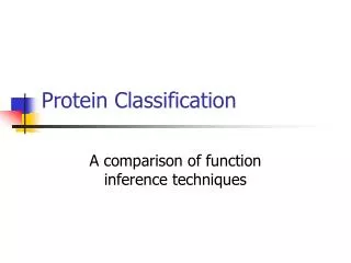
Protein Classification

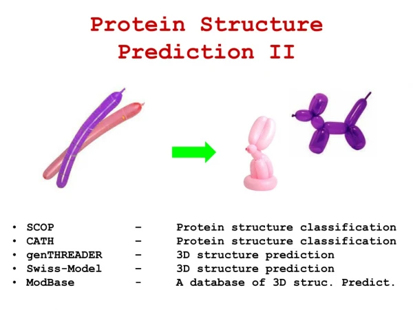
Protein Classification

Protein Classification • Given a new protein, can we place it in its “correct” position within an existing protein hierarchy? Methods • BLAST / PsiBLAST • Profile HMMs • Supervised Machine Learning methods Fold Superfamily new protein ? Family Proteins

PSI-BLAST Given a sequence query x, and database D • Find all pairwise alignments of x to sequences in D • Collect all matches of x to y with some minimum significance • Construct position specific matrix M • Each sequence y is given a weight so that many similar sequences cannot have much influence on a position (Henikoff & Henikoff 1994) • Using the matrix M, search D for more matches • Iterate 1–4 until convergence Profile M

Dm-1 Dm-1 Dm-1 Dm Dm Dm D1 D1 D1 D2 D2 D2 BEGIN BEGIN BEGIN END END END I0 I0 I0 I1 I1 I1 Im-1 Im-1 Im-1 Im Im Im M1 M1 M1 M2 M2 M2 Mm Mm Mm Classification with Profile HMMs Fold Superfamily Family new protein ?

Dm-1 Dm D1 D2 BEGIN END I0 I1 Im-1 Im M1 M2 Mm The Fisher Kernel • Fisher score • UX =  log P(X | H1, ) • Quantifies how each parameter contributes to generating X • For two different sequences X and Y, can compare UX, UY • D2F(X, Y) = ½ 2 |UX – UY|2 • Given this distance function, K(X, Y) is defined as a similarity measure: • K(X, Y) = exp(-D2F(X, Y)) • Set  so that the average distance of training sequences Xi  H1 to sequences Xj  H0 is 1

The Fisher Kernel • To train a classifier for a given family H1, • Build profile HMM, H1 • UX =  log P(X | H1, ) (Fisher score) • D2F(X, Y) = ½ 2 |UX – UY|2 (distance) • K(X, Y) = exp(-D2F(X, Y)), (akin to dot product) • L(X) = XiH1i K(X, Xi) –XjH0j K(X, Xj) • Iteratively adjust  to optimize J() = XiH1i(2 - L(Xi))–XjH0j(2 + L(Xj)) • To classify query X, • Compute UX • Compute K(X, Xi) for all training examples Xi with I≠ 0 (few) • Decide based on L(X) >? 0

O. Jangmin

QUESTION Running time of Fisher kernel SVM on query X?

k-mer based SVMs Leslie, Eskin, Weston, Noble; NIPS 2002 Highlights • K(X, Y) = exp(-½ 2 |UX – UY|2), requires expensive profile alignment: UX =  log P(X | H1, ) – O(|X| |H1|) • Instead, new kernel K(X, Y) just “counts up” k-mers with mismatches in common between X and Y – O(|X|) in practice • Off-the-shelf SVM software used

X Y k-mer based SVMs • For given word size k, and mismatch tolerance l, define K(X, Y) = # distinct k-long word occurrences with ≤ l mismatches • Define normalized kernel K’(X, Y) = K(X, Y)/ sqrt(K(X,X)K(Y,Y)) • SVM can be learned by supplying this kernel function A B A C A R D I K(X, Y) = 4 K’(X, Y) = 4/sqrt(7*7) = 4/7 Let k = 3; l = 1 A B R A D A B I

SVMs will find a few support vectors After training, SVM has determined a small set of sequences, the support vectors, who need to be compared with query sequence X v

Benchmarks

Semi-Supervised Methods GENERATIVE SUPERVISED METHODS

Semi-Supervised Methods DISCRIMINATIVE SUPERVISED METHODS

Semi-Supervised Methods UNSUPERVISED METHODS Mixture of Centers Data generated by a fixed set of centers (how many?)

Semi-Supervised Methods • Some examples are labeled • Assume labels vary smoothly among all examples

Semi-Supervised Methods • Some examples are labeled • Assume labels vary smoothly among all examples • SVMs and other discriminative methods may make significant mistakes due to lack of data

Semi-Supervised Methods • Some examples are labeled • Assume labels vary smoothly among all examples Attempt to “contract” the distances within each cluster while keeping intracluster distances larger

Semi-Supervised Methods • Kuang, Ie, Wang, Siddiqi, Freund, Leslie 2005 • A Psi-BLAST profile—based method • Weston, Leslie, Elisseeff, Noble, NIPS 2003 • Cluster kernels

(semi)1. Profile k-mer based SVMs PSI-BLAST • For each sequence X, • Obtain PSI-BLAST profile Q(X) = {pi(); : amino acid, 1≤ i ≤ |X|} • For every k-mer in X, xj … xj+k-1, define -neighborhood Mk, (Q[xj…xj+k-1]) = {b1…bk | -i=0…k-1 log pj+i(bi) < } • Define K(X, Y) For each b1…bk matching m times in X, n times in Y, add m*n • In practice, each k-mer can have ≤ 2 mismatches and K(X, Y) can be computed quickly in O(k2 202 (|X| + |Y|)) Profile M

(semi)1. Discriminative motifs • According to this kernel K(X, Y), sequence X is mapped to Φk,(X): vector in 20k dimensions • Φk,(X)(b1…bk) = # k-mers in Q(X) whose neighborhood includes b1…bk • Then, SVM learns a discriminating “hyperplane” with normal vector v: • v = i=1…N (+/-) iΦk,(X(i)) • Consider a profile k-mer Q[xj…xj+k-1]; its contribution to v is ~ • Φk,(Q[xj…xj+k-1]), v • Consider a position i in X: count up the contributions of all words containing xi • g(xi) = j=1…kmax{ 0, Φk,(Q[xi-k+j…xj-1+j]), v} • Sort these contributions within all positions of all sequences, to pick important positions or discriminative motifs

(semi)1. Discriminative motifs • Consider a position i in X: count up the contributions to v of all words containing xi • Sort these contributions within all positions of all sequences, to pick discriminative motifs

(semi)2. Cluster Kernels • Two (more!) methods • Neighborhood • For each X, run PSI-BLAST to get similar seqs  Nbd(X) • Define Φnbd(X) = 1/|Nbd(X)| X’  Nbd(X)Φoriginal(X’) “Counts of all k-mers matching with at most 1 diff. all sequences that are similar to X” • Knbd(X, Y) = 1/(|Nbd(X)|*|Nbd(Y)) X’  Nbd(X)Y’  Nbd(Y) K(X’, Y’) • Bagged mismatch

(semi)2. Cluster Kernels • Two (more!) methods • Neighborhood • For each X, run PSI-BLAST to get similar seqs  Nbd(X) • Define Φnbd(X) = 1/|Nbd(X)| X’  Nbd(X)Φoriginal(X’) “Counts of all k-mers matching with at most 1 diff. all sequences that are similar to X” • Knbd(X, Y) = 1/(|Nbd(X)|*|Nbd(Y)) X’  Nbd(X)Y’  Nbd(Y) K(X’, Y’) • Bagged mismatch • Run k-means clustering n times, giving p = 1,…,n assignments cp(X) • For every X and Y, count up the fraction of times they are bagged together Kbag(X, Y) = 1/n p 1(cp(X) = cp (Y)) • Combine the “bag fraction” with the original comparison K(.,.) Knew(X, Y) = Kbag(X, Y) K(X, Y)

Some Benchmarks

Google-like homology search • The internet and the network of protein homologies have some similarity—scale free • Given query X, Google ranks webpages by a flow algorithm • From each webpage W, linked nbrs receive flow • At time t+1, W sends to nbrs flow it received at time t • Finite, ergodic, aperiodic Markov Chain • Can find stationary distribution efficiently as left eigenvector with eigenvalue 1 • Start with arbitrary probability distribution, and multiply by the transition matrix

Google-like homology search Weston, Elisseeff, Zhu, Leslie, Noble, PNAS 2004 RANKPROP algorithm for protein homology • First, compute a matrix Kij of PSI-BLAST homology between proteins i and j, normalized so that jKji = 1 • Initialization y1(0) = 1; yi(0) = 0 • For t = 0, 1, …, • For i = 2 to m • yi(t+1) = K1i + Kjiyj(t) In the end, let yi be the ranking score for similarity of sequence i to sequence 1 ( = 0.95 is good)

Google-like homology search For a given protein family, what fraction of true members of the family are ranked higher than the first 50 non-members?

Protein Structure Prediction

Protein Structure Determination • Experimental • X-ray crystallography • NMR spectrometry • Computational – Structure Prediction (The Holy Grail) Sequence implies structure, therefore in principle we can predict the structure from the sequence alone

Protein Structure Prediction • ab initio • Use just first principles: energy, geometry, and kinematics • Homology • Find the best match to a database of sequences with known 3D-structure • Threading • Meta-servers and other methods

Ab initio Prediction • Sampling the global conformation space • Lattice models / Discrete-state models • Molecular Dynamics • Picking native conformations with an energy function • Solvation model: how protein interacts with water • Pair interactions between amino acids • Predicting secondary structure • Local homology • Fragment libraries

Lattice String Folding • HP model: main modeled force is hydrophobic attraction • NP-hard in both 2-D square and 3-D cubic • Constant approximation algorithms • Not so relevant biologically

Lattice String Folding

Protein Classification