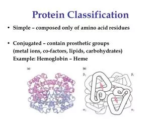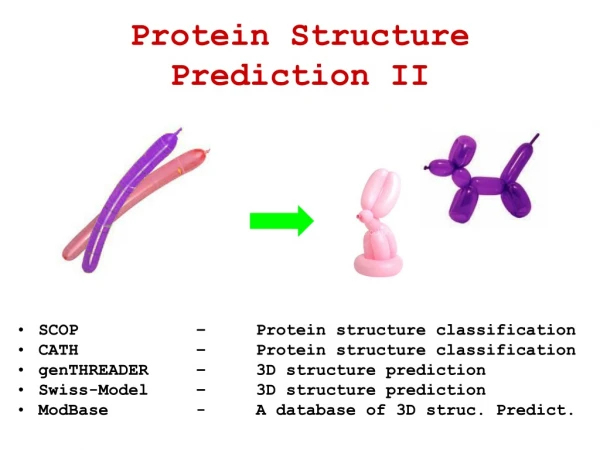
Protein Classification
Protein Classification. PDB Growth. New PDB structures. Protein classification. Number of protein sequences grow exponentially Number of solved structures grow exponentially Number of new folds identified very small (and close to constant) Protein classification can

Protein Classification
E N D
Presentation Transcript
PDB Growth New PDB structures
Protein classification • Number of protein sequences grow exponentially • Number of solved structures grow exponentially • Number of new folds identified very small (and close to constant) • Protein classification can • Generate overview of structure types • Detect similarities (evolutionary relationships) between protein sequences Morten Nielsen,CBS, BioCentrum, DTU
Protein world Protein structure classification Protein fold Protein superfamily Protein family Morten Nielsen,CBS, BioCentrum, DTU
Structure Classification Databases • SCOP • Manual classification (A. Murzin) • scop.berkeley.edu • CATH • Semi manual classification (C. Orengo) • www.biochem.ucl.ac.uk/bsm/cath • FSSP • Automatic classification (L. Holm) • www.ebi.ac.uk/dali/fssp/fssp.html Morten Nielsen,CBS, BioCentrum, DTU
Major classes in SCOP • Classes • All alpha proteins • Alpha and beta proteins (a/b) • Alpha and beta proteins (a+b) • Multi-domain proteins • Membrane and cell surface proteins • Small proteins Morten Nielsen,CBS, BioCentrum, DTU
All a: Hemoglobin (1bab) Morten Nielsen,CBS, BioCentrum, DTU
All b: Immunoglobulin (8fab) Morten Nielsen,CBS, BioCentrum, DTU
a/b:Triosephosphate isomerase (1hti) Morten Nielsen,CBS, BioCentrum, DTU
a+b: Lysozyme (1jsf) Morten Nielsen,CBS, BioCentrum, DTU
Families • Proteins whose evolutionarily relationship is readily recognizable from the sequence (>~25% sequence identity) • Families are further subdivided into Proteins • Proteins are divided into Species • The same protein may be found in several species Fold Superfamily Family Proteins Morten Nielsen,CBS, BioCentrum, DTU
Superfamilies • Proteins which are (remote) evolutionarily related • Sequence similarity low • Share function • Share special structural features • Relationships between members of a superfamily may not be readily recognizable from the sequence alone Fold Superfamily Family Proteins Morten Nielsen,CBS, BioCentrum, DTU
Folds • Proteins which have >~50% secondary structure elements arranged the in the same order in the protein chain and in three dimensions are classified as having the same fold • No evolutionary relation between proteins Fold Superfamily Family Proteins Morten Nielsen,CBS, BioCentrum, DTU
Protein Classification • Given a new protein, can we place it in its “correct” position within an existing protein hierarchy? Methods • BLAST / PsiBLAST • Profile HMMs • Supervised Machine Learning methods Fold Superfamily new protein ? Family Proteins
PSI-BLAST Given a sequence query x, and database D • Find all pairwise alignments of x to sequences in D • Collect all matches of x to y with some minimum significance • Construct position specific matrix M • Each sequence y is given a weight so that many similar sequences cannot have much influence on a position (Henikoff & Henikoff 1994) • Using the matrix M, search D for more matches • Iterate 1–4 until convergence Profile M
Dm-1 Dm D1 D2 BEGIN END I0 I1 Im-1 Im M1 M2 Mm Profile HMMs • Each M state has a position-specific pre-computed substitution table • Each I and D state has position-specific gap penalties • Profile is a generative model: • The sequence X that is aligned to H, is thought of as “generated by” H • Therefore, H parameterizes a conditional distribution P(X | H) Protein profile H
Dm-1 Dm-1 Dm-1 Dm Dm Dm D1 D1 D1 D2 D2 D2 BEGIN BEGIN BEGIN END END END I0 I0 I0 I1 I1 I1 Im-1 Im-1 Im-1 Im Im Im M1 M1 M1 M2 M2 M2 Mm Mm Mm Classification with Profile HMMs Fold Superfamily Family new protein ?
Classification with Profile HMMs • How generative models work • Training examples ( sequences known to be members of family ): positive • Model assigns a probability to any given protein sequence. • The sequence from that family yield a higher probability than that of outside family. • Log-likelihood ratio as score P(X | H1) P(H1) P(H1|X) P(X) P(H1|X) L(X) = log -------------------------- = log --------------------- = log -------------- P(X | H0) P(H0) P(H0|X) P(X) P(H0|X)
Generation of a protein by a profile HMM P(X | H) ?? To generate sequence x1…xn by profile HMM H: We will find the sum probability of all possible ways to generate X • Define • AjM(i): probability of generating x1…xi and ending with xi being emitted from Mj • AjI(i): probability of generating of x1…xi and ending with xi being emitted from Ij • AjD(i): probability of generating of x1…xi and ending in Dj • (xi is the last character emitted before Dj)
Alignment of a protein to a profile HMM AjM(i) = εM(j)(xi) * { Aj-1M(i – 1) + log αM(j-1)M(j) + Aj-1I(i – 1) + log αI(j-1)M(j) + Aj-1D(i – 1) + log αD(j-1)M(j) } AjI(i) = εI(j)(xi) * { AjM(i – 1) + log αM(j)I(j) + AjI(i – 1) + log αI(j)I(j) + AjD(i – 1) + log αD(j)I(j) } AjD(i) = { Aj-1M(i) + log αM(j-1)D(j) + Aj-1I(i) + log αI(j-1)D(j) + Aj-1D(i) + log αD(j-1)D(j) }
Discriminative Methods Instead of modeling the process that generates data, directly discriminate between classes • More direct way to the goal • Better if model is not accurate
Discriminative Models -- SVM • If x1 … xn training examples, • sign(iixiTx) “decides” where x falls • Train i to achieve best margin margin Decision Rule: red: vTx > 0 v Large Margin for |v| < 1 Margin of 1 for small |v|
Discriminative protein classification Jaakkola, Diekhans, Haussler, ISMB 1999 • Define the discriminating function to be L(X) = XiH1 i K(X, Xi) - XjH0 j K(X, Xj) We decide X family H whenever L(X) > 0 • For now, let’s just assume K(.,.) is a similarity function • Then, we want to train i so that this classifier makes as few mistakes as possible in the new data • Similarly to SVMs, train i so that margin is largest for 0 i 1
Discriminative protein classification • Ideally, for training examples, L(Xi) ≥ 1 if Xi H1, L(Xi) -1 otherwise • This is not always possible; softer constraints are obtained with the following objective function J() = XiH1 i(2 - L(Xi)) - XjH0 j(2 + L(Xj)) • Training: for Xi H, try to “make” L(Xi) = 1 1 - L(Xi) + i K(Xi, Xi) • i -----------------------------; with minimum allowable value 0, and maximum 1 K(Xi, Xi) • Similarly, for Xi H0 try to “make” L(Xi) = -1
Dm-1 Dm D1 D2 BEGIN END I0 I1 Im-1 Im M1 M2 Mm The Fisher Kernel • The function K(X, Y) compares two sequences • Acts effectively as an inner product in a (non-Euclidean) space • Called “Kernel” • Has to be positive definite • For any X1, …, Xn, the matrix K: Kij = K(Xi, Xj) is such that For any X Rn, X≠ 0, XT K X > 0 • Choice of this function is important • Consider P(X | H1, ) – sufficient statistics • How many expected times X takes each transition/emission
Dm-1 Dm D1 D2 BEGIN END I0 I1 Im-1 Im M1 M2 Mm The Fisher Kernel • Fisher score • UX = log P(X | H1, ) • Quantifies how each parameter contributes to generating X • For two different sequences X and Y, can compare UX, UY • D2F(X, Y) = ½ 2 |UX – UY|2 • Given this distance function, K(X, Y) is defined as a similarity measure: • K(X, Y) = exp(-D2F(X, Y)) • Set so that the average distance of training sequences Xi H1 to sequences Xj H0 is 1 Question: Is partial derivative larger when X “uses” a given parameter I more or less often? Question: Is partial derivative larger when a given parameter I is larger or smaller?
The Fisher Kernel • In summary, to distinguish between family H1 and (non-family) H0, define • Profile H1 • UX = log P(X | H1, ) (Fisher score) • D2F(X, Y) = ½ 2 |UX – UY|2 (distance) • K(X, Y) = exp(-D2F(X, Y)), (akin to dot product) • L(X) = XiH1i K(X, Xi) –XjH0j K(X, Xj) • Iteratively adjust to optimize • J() = XiH1i(2 - L(Xi))–XjH0j(2 + L(Xj))
Dm-1 Dm-1 Dm Dm D1 D1 D2 D2 BEGIN BEGIN END END I0 I0 I1 I1 Im-1 Im-1 Im Im M1 M1 M2 M2 Mm Mm The Fisher Kernel • If a given superfamily has more than one profile model, • Lmax(X) = maxi Li(X) = maxi(XjHij K(X, Xj) –XjH0j K(X, Xj)) Superfamily Family
Benchmarks • Methods evaluated • BLAST (Altschul et al. 1990; Gish & States 1993) • HMMs using SAM-T98 methodology (Park et al. 1998; Karplus, Barrett, & Hughey 1998; Hughey & Krogh 1995, 1996) • SVM-Fisher • Measurement of recognition rate for members of superfamilies of SCOP (Hubbard et al. 1997) • PDB90 eliminates redundant sequences • Withhold all members of a given SCOP family • Train with the remaining members of SCOP superfamily • Test with withheld data • Question: “Could the method discover a new family of a known superfamily?” O. Jangmin
Other methods • WU-BLAST version 2.0a16 (Althcshul & Gish 1996) • PDB90 database was queried with each positive training examples, and E-values were recorded. • BLAST:SCOP-only • BLAST:SCOP+SAM-T98-homologs • Scores were combined by the maximum method • SAM-T98 method • Same data and same set of models as in the SVM-Fisher • Combined with maximum methods O. Jangmin
Results • Metric : the rate of false positives (RFP) • RFP for a positive test sequence : the fraction of negative test sequences that score as good of better than positive sequence • Result of the family of the nucleotide triphosphate hydrolases SCOP superfamily • Test the ability to distinguish 8 PDB90 G proteins from 2439 sequences in other SCOP folds O. Jangmin
Table 1. Rate of false positives for G proteins family. BLAST = BLAST:SCOP-only, B-Hom = BLAST:SCOP+SAMT-98-homologs, S-T98 = SAMT-98, and SVM-F = SVM-Fisher method O. Jangmin
QUESTION Running time of Fisher kernel SVM on query X?