Download
1 / 28
280 likes | 413 Vues
Modeling Menstrual Cycle Length in Pre- and Peri-Menopausal Women. Michael Elliott Xiaobi Huang Sioban Harlow University of Michigan School of Public Health September 30, 2008. Outline. Has the onset of menopause changed since the early 20 th Century?

E N D
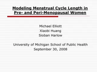
Modeling Menstrual Cycle Length in Pre- and Peri-Menopausal Women Michael Elliott Xiaobi Huang Sioban Harlow University of Michigan School of Public Health September 30, 2008
Outline Has the onset of menopause changed since the early 20th Century? Tremin I: U. Minnesota Undergraduates 1930’s. Tremin II: U. Minnesota Undergraduates 1960’s. Develop statistical model for menstrual cycle length. Bayesian methods Apply to complete data from Tremin I. Future work Accounting for missing data (hormone, dropout). Including Tremin II data. Relating to existing suggestions for FMP markers (60 days, 90 days, etc.).
Characterized by: Stable trend during a woman’s 20’s and 30’s “Breakdown” several months to several years before FMP Increase in variability Increase in mean length Modeling Menstrual Cycle Length: Observed Data
Easier to see on a log scale: Modeling Menstrual Cycle Length: Observed Data
There appears to be a common pattern to how menstrual cycle length changes over age. A linear changepoint model: Can be implemented as a linear spline with one changepoint: , where Modeling Menstrual Cycle Length: Linear Changepoint Model
Different slopes and intercepts either side of θ: But means converge at the “knot” of θ: Modeling Menstrual Cycle Length: Linear Changepoint Model
Variance can be modeled via linear changepoint model, just like the mean. Note that the changepoint(s) θare estimated from the data, not fixed in advance. Modeling Menstrual Cycle Length: Linear Changepoint Model
Despite general overall pattern being the same, women have unique ages when their cycle lengths begin to change, as well as difference means and variances at “baseline”. This suggests constructing a hierarchical model in which women will have unique parameters governing mean and variance changepoint models. Modeling Menstrual Cycle Length: Hierarchical Model
Start at age 35 and take log of cycle length to improve normal approximation. Linear changepoint for both mean and variance where is the length in days of the tth menstrual cycle for the ith woman, , is her age in years at the start of her tth cycle, and Modeling Menstrual Cycle Length: Hierarchical Model
Each of the individual parameters is then assumed to follow a common distribution: where . Allows information about cycle parameters to be shared across women. Accommodates “within-woman” correlation in cycle lengths Relates cycle parameters to baseline covariates via regression coefficients . Modeling Menstrual Cycle Length: Hierarchical Model
Considering a model of this form is easier from a Bayesian perspective. Classical or “frequentist" approach to statistics considers observed data y to be random, governed by fixed (unknown) parameters θ. Determine the joint distribution of . and consider as a function of θ: . Point estimate of made by maximizing or . Inference about θ made by considering repeated sampling properties of y for different θ. Ex: 95% confidence interval, a hypothetical set of which will contain θ with 95% probability Bayesian Models
Bayesian statistics also models , but considers θto have a probability distribution of its own, . Prior information contained in is updated from data y to obtain a posterior distribution of θ: Hierarchical models model prior parameters with “hyperprior” distributions : Bayesian Models
Prior distributions or hyperprior distributions encode prior knowledge about parameters, but can be chosen to be very weakly informative if little prior information is available, or if it is to be ignored. Here Modern computational techniques such as Markov Chain Monte Carlo allow complex models such as those to be used here to be fit (relatively) painlessly. Results from 3,000 draws of Gibbs sampler, 1,000 draws discarded after “burn-in”. Bayesian Models
Fit the above model to the 106 women with complete data in Tremin I. Pregnancies, abortions. No hormone use or gaps in reporting. Subject level parameters (random effects). Fit of predicted means and variances. Regression against parity, menarche, means and standard errors at age 25-29. Correlation of subject-level parameters. Results
Mean cycle length: Posterior mean (95% posterior predictive interval) 2.5 and 97.5 Percentiles: Posterior mean (95% PPI) Results: Subject-level estimates of trends
One-changepoint model provides reasonably good fit to the data. Subject-level differences in mean and variance trends appear to be captured. Uncertainty in the location of the changepoints reflected in the smoothness of the ``elbow’’ for the mean and variances. Results: Subject-level estimates of trends
Posterior means and 80% posterior predictive intervals for mean changepoint and variance changepoint. Variability in cycle length increases well in advance of increases in mean cycle length itself. Changepoints for some subjects are well-estimated, while there is a great deal of uncertainty for others. Results: Subject-level estimates of trends
Results: Population Mean for trend parameters (adjusted for parity, age at menarche, and mean and variance of cycles at age 25-29)
Parity not associated with cycle structure. Weak evidence that earlier menarche associated with increasing variability before changepoint. Higher historical mean: Higher mean at 35. Decline in variability before changepoint. Later changepoints for both mean and variance. Higher historical variance: Lower mean at 35. Earlier changepoints for both mean and variance. Results: Population Mean for trend parameters (adjusted for parity, age at menarche, and mean and variance of cycles at age 25-29)
Longer cycles at age 35 are associated with somewhat later changepoints in both mean and variance. Highly variable cycles at age 35 are associated with slower increases/declines in variability before their variability changepoint, but more rapid increases thereafter. Later mean changepoints are associated with slower increases or even declines in variability before their variability changepoint, and slower increases thereafter. Later mean changepoints are strongly associated with later variance changepoints. Results: Correlations among random effects
Account for missing data (hormone, dropout). Impute missing cycles under model, and then obtain draws from posterior distribution of parameters conditional on observed and imputed data. Use results from alternative non-model-based approaches Next Steps: Modeling
Model checking “Eyeball” approach shows good fit Formalize with posterior predictive checks. Generate predictive data under model and compute posterior distributions of statistics of interest (chi-square measures, etc.) Compare with posterior distribution of statistics using observed (fixed) data. Next Steps: Modeling
Include Tremin II data. Add as covariate to population model Assess secular trends pre- and post- birth control use. Next Steps: Analysis
Relate to existing suggestions for FMP markers (60 days, 90 days, etc.). Consider predictive value of model for pre-FMP subjects. “Cross-validation” with Tremin data. Validation with other data sources. Next Steps: Analysis
Look for cycle behavior that might be reflective of disease Next Steps: Analysis