4.3 Least-Squares Regression
190 likes | 225 Vues
Learn about regression lines, prediction methods, and the LSRL in statistics, key facts and correlations. Helpful tips for fitting lines and interpreting data patterns in a straightforward manner.

4.3 Least-Squares Regression
E N D
Presentation Transcript
4.3 Least-Squares Regression • Regression Lines • Least-Squares Regression Line • Facts about Least-Squares Regression • Correlation and Regression
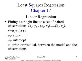
Example: Predict the number of new adult birds that join the colony based on the percent of adult birds that return to the colony from the previous year. If 60% of adults return, how many new birds are predicted? Regression Line A regression lineis a straight line that describes how a response variable y changes as an explanatory variable x changes. We can use a regression line to predict the value of y for a given value of x.
The regression line • A regression line is a straight line drawn through the data points that describes how a response variable y changes as an explanatory variable x changes - the description is made through the slope and intercept of the line. • We often use a regression line to predict the value of y for a given value of x; the line is also called the prediction line, or the least-squares line, or the best fit line and it is said that we have “Fit a line” to the data. • In regression, the distinction between explanatory and response variables is important - if you interchange the roles of x and y, the regression line is different. y-hat is the predicted value of y b1 is the slope b0 is the y-intercept
Regression Line When a scatterplot displays a linear pattern, we can describe the overall pattern by drawing a straight line through the points. Fitting a line to data means drawing a line that comes as close as possible to the points. • x is the value of the explanatory variable. • y-hat is the predicted value of the response variable for a given value of x. • b1is the slope, the amount by which the predicted y changes for each one-unit increase in x. • b0is the intercept, the value of the predicted y when x = 0. Regression equation: y-hat = b0 + b1x
Least-Squares Regression Line Least-Squares Regression Line (LSRL) • The least-squares regression line of y on x is the line that minimizes the sum of the squares of the vertical distances of the data points from the line. • If we have data on an explanatory variable x and a response variable y, the equation of the least-squares regression line is: • y-hat= b0 + b1x Since we are trying to predict y, we want the regression line to be as close as possible to the data points in the vertical (y) direction.
How to: First we calculate the slope of the line, b1; from statistics we already know: r is the correlation. sy is the standard deviation of the response variable y. sx is the the standard deviation of the explanatory variable x. Once we know b1, the slope, we can calculate b0, the y-intercept: Where and are the sample means of the x and y variables Typically, we use the TI-83 or JMP (Analyze -> Fit Y by X -> under the red triangle, Fit Line) to compute the b's, rarely using the above formulas…but notice what you can learn from them…
JMP output – For example 4.16 Do this example! the regression line intercept estimate is b0 slope estimate b1 is the coefficient (Estimate) of the NEA term
Facts about Least-Squares Regression Regression is one of the most common statistical settings, and least- squares is the most common method for fitting a regression line to data. Here are some facts about least-squares regression lines – see slide #6 above! • Fact 1: A change of one standard deviation in x corresponds to a change of r standard deviations in y. • Fact 2: The LSRL always passes through (x-bar, y-bar). • Fact 3: The distinction between explanatory and response variables is essential.
Correlation and Regression Least-squares regression looks at the distances of the data points from the line only in the y direction. The variables x and y play different roles in regression. Even though correlation r ignores the distinction between x and y, there is a close connection between correlation and regression. The square of the correlation, r2, is the fraction of the variation in the values of y that is explained by the least-squares regression of y on x. • r2is called the coefficient of determination.
r = 0.87 r 2 = 0.76 Coefficient of determination, r 2 r 2, the coefficient of determination, is the square of the correlation coefficient. r 2 representsthe percentage of the variation in y(vertical scatter from the regression line) that can be explained by the regression of y on x.r 2 is the ratio of the variance of the predicted values of y (y-hats - as if no scatter around the line) to the variance of the actual values of y.
HW: Read sections 4.3 and 4.4 Do #4.53-4.56, 4.58 and 4.69; use JMP to compute the regression line and the correlation coefficient and its square.
4.4 Cautions about Correlation and Regression • Residuals and Residual Plots • Outliers and Influential Observations • Lurking Variables • Correlation and Causation
Residuals A regression line describes the overall pattern of a linear relationship between an explanatory variable and a response variable. Deviations from the overall pattern are also important. The vertical distances between the points and the least-squares regression line are called residuals. A residualis the difference between an observed value of the response variable and the value predicted by the regression line: residual = observed y – predicted y
Residual Plots • A residual plotis a scatterplot of the regression residuals against the explanatory variable. Residual plots help us assess the fit of a regression line. • Look for a “random” scatter around zero. • Residual patterns suggest deviations from a linear relationship. Gesell Adaptive Score and Age at First Word
Outliers and Influential Points • Outliers in the x direction are often influentialfor the least-squares regression line, meaning that the removal of such points would markedly change the equation of the line. An outlieris an observation that lies outside the overall pattern of the other observations. • Outliers in the ydirection have large residuals.
After removing child 18 From all of the data Outliers and Influential Points Gesell Adaptive Score and Age at First Word r2 = 11% r2 = 41% Chapter 5
Sarah’s height was plotted against her age. Can you predict her height at age 42 months? Can you predict her height at age 30 years (360 months)? Extrapolation
Regression line:y-hat = 71.95 + 0.383 x Height at age 42 months? y-hat = 88 Height at age 30 years? y-hat = 209.8 She is predicted to be 6’10.5” at age 30! Extrapolation
Cautions about Correlation and Regression • Both describe linear relationships. • Both are affected by outliers. • Always plot the data before interpreting. • Beware of extrapolation. • Predicting outside of the range of x • Beware of lurking variables. • These have an important effect on the relationship among the variables in a study, but are not included in the study. • Correlation does not imply causation!