System Function of discrete-time systems

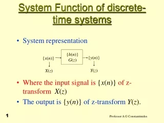
1. {h(n)} G(z) {y(n)} {x(n)} Y(z) X(z) System Function of discrete-time systems • System representation • Where the input signal is{x(n)}ofz-transformX(z) • The output is {y(n)} of z-transform Y(z). 1

2. System Function of discrete-time systems • The system has an impulse response h(n) • Define so that and hence • Clearly when X(z) = 1 then G(z) = Y(z) i.e. G(z) is the z-transform of the impulse response h(n) 2

3. Frequency Response • Let the input be • Then the output is • Where • and 3

4. System Function of discrete-time systems • However • While the amplitude & phase responses are • And hence 4

5. System Functions-Amplitude response • Evidently • And hence • Thus • ie for real systems amplitude is an even function, and phase an odd function of frequency 5

6. System Functions-Amplitude response • Moreover from • Since at is finite we obtain 6

7. System Functions-Phase response • From • At we have • Thus for real systems the amplitude response must approach zero frequency with zero slope, while the phase rsponse must be zero at the origin 7

8. System Functions-Phase response • For , • Hence 8

9. System Functions-Group delay • Thus • where 9

10. Suppression of a frequency band • A real rational transfer function H(z) cannot suppress a band of frequencies completely. i.e.cannot be identically zero for in • This may be demonstrated as follows 10

11. System Function of discrete-time systems • To produce a zero at say we must have in the numerator of H(z) a factor of the form • Therefore for one zero in the band the factor is • and since there are an infinite number of points in the band we need factors in the numerator as 11

12. System Function of discrete-time systems • Clearly the result is not a rational function • Hence it cannot be the transfer function of a digital signal processing system. 12

13. Stability Test • For stability a DSP transfer function must have poles inside the unit circle on the z-plane. • We need to have a means of determining whether the denominator of a given transfer function has all its zeros inside the unit circle. • The procedures for doing so are called stability tests. 13

14. Stability Test • Let the transfer function to be tested be • where n is the order of the transfer function. Set A = 1. • For stability Dn(z) must have no zeros in the region 14

15. Stability Test • Consider the simple case of a quadratic denominator • Rewrite as (ignore the factor ) • If the roots are complex, say then 15

16. Stability Test • Thus and • For stability and thus • For real roots • If choose root with largest absolute value and make less than 1 16

17. Stability Test • Thus • And since quantities are positive we obtain • Similarly for • Thus jointly we have 17

18. Stability Test • These conditions form the Stability Triangle Stability region inside triangle 18

19. Stability Test • For higher order functions most tests rely on an iterative precedure that involves • reduction of the polynomial degree by unity • a simple test • Jury-Marden Test: We write Dn(z) as • where is a constant chosen to make of degree (n - 1) 19

20. Stability Test • Repeat equation • Hence • And thus • Set so that is of degree (n-1) when 20

21. Stability Test • Rouche’s Theorem: If the polynomials and are such that in the same region then has the same number of zeros in that region as 21

22. Stability Test • we observe that Dn(z) has as many zeros as either or depending on whether • or • Ie or 22

23. Stability Test • Thus if then is unstable as it has as many zeros as which has at most (n - 1) zeros within |z| < 1. • If then can have as many zeros within |z| < 1 as • The zero at z = 0 can be removed and the procedure repeated for the remaining polynomial 23

24. Stability Test • An alternative test: Consider • So that • For this equation to be a polynomial we require the constant term in the numerator to bezeroso as to be able to cancel through a factorz 24

25. Stability Test • Thus or • The rest of the argument is similar to the previous case 25

26. Further Stability Test • Given that and show that on the unit circle for any real • Construct • Repeat the previous arguments 26

27. Digital Two-Pairs • The LTI discrete-time systems considered so far are single-input, single-output • Often such systems can be efficiently realised by interconnecting two-input, two-output structures, known as two-pairs 27

28. Digital Two-Pairs • Figures below show two commonly used block diagram representations of a two-pair • Here and denote the two outputs, and and denote the two inputs, where the dependencies on the variablezhas been omitted for simplicity 28

29. t Digital Two-Pairs • The input-output relation of a digital two-pair is given by • In the above relation the matrixtgiven by is called thetransfer matrixof the two-pair 29

30. G - - Digital Two-Pairs • An alternate characterisation of the two-pair is in terms of its chain parameters as where the matrix G given by is called the chain matrix of the two-pair 30

31. Digital Two-Pairs • The transfer and chain parameters are related as 31

32. - - - - Two-Pair Interconnections Cascade Connection - G-cascade • Here 32

33. Two-Pair Interconnections • But from figure, and • Substituting the above relations in the first equation on the previous slide and combining the two equations we get • Hence, 33

34. - - - - Two-Pair Interconnections Cascade Connection - t-cascade • Here 34

35. Two-Pair Interconnections • But from figure, and • Substituting the above relations in the first equation on the previous slide and combining the two equations we get • Hence, 35

36. G(z) Two-Pair Interconnections Constrained Two-Pair • It can be shown that H(z) 36