Exploring Ice Ages: Earth's Orbital Changes and Glacial Evidence
560 likes | 675 Vues
Delve into the Quaternary period, ice volume indicators, orbit fluctuations, and their correlation with glaciers. Learn about oxygen isotopes, global ice volume, sediment core analysis, and factors affecting d18O variations.

Exploring Ice Ages: Earth's Orbital Changes and Glacial Evidence
E N D
Presentation Transcript
Topic Outline • Introduction to the Quaternary • Oxygen isotopes as an indicator of ice volume • Temporal variations in ice volume • Periodic changes in Earth’s orbit • Relationship between orbital changes and variations in ice volume
Topic Outline • Introduction to the Quaternary • Oxygen isotopes as an indicator of ice volume • Temporal variations in ice volume • Periodic changes in Earth’s orbit • Relationship between orbital changes and variations in ice volume
The Quaternary Period • In the first half of the 19th century, Louis Agassiz argued that widespread glaciation was the explanation for various unusual geologic features in much of North America and Europe. • A lengthy scientific debate ensued, but the evidence for a number of continental glaciations gradually became accepted.
Moraines • As a glacier advances, its leading edge acts like the blade of a bulldozer, pushing rock and debris in advance. • These remnants of glaciation, called terminal moraines, mark the location of maximum ice extent.
Moraines • As a glacier advances, its leading edge acts like the blade of a bulldozer, pushing rock and debris in advance. • These remnants of glaciation, called terminal moraines, mark the location of maximum ice extent.
Moraines • As a glacier advances, its leading edge acts like the blade of a bulldozer, pushing rock and debris in advance. • These remnants of glaciation, called terminal moraines, mark the location of maximum ice extent.
LGM Ice Extent in the Northeastern United States Moraines from earlier glaciations are most often destroyed by subsequent glaciations, so moraines are generally evidence of the most recent glacial advance.
Topic Outline • Introduction to the Quaternary • Oxygen isotopes as an indicator of ice volume • Temporal variations in ice volume • Periodic changes in Earth’s orbit • Relationship between orbital changes and variations in ice volume
Oxygen Isotopes • A small fraction of water molecules contain the heavy isotope 18O instead of 16O. • 18O/16O ≈ 1/500 • This ratio is not constant, but varies over a range of several percent. • Vapor pressure of H218O is lower than that of H216O, thus the latter is more easily evaporated.
d18O • As water vapor is transported poleward in the hydrologic cycle, each cycle of evaporation and condensation lowers the ratio of H218O to H216O, in a process called fractionation. • This ratio is expressed as d18O.
d18Ovs. Temperature • As a consequence of fractionation, d18O in precipitation decreases with decreasing temperature. • Ice sheets have very low d18O values. Observed d18O in average annual precipitation as a function of mean annual air temperature (Dansgaard 1964). Note that all the points in this graph are for high latitudes (>45°). (From Broecker 2002)
d18O and Global Ice Volume • As ice sheets grow, the water removed from the ocean has lower d18O than the water that remains. • Thus the d18O value of sea water in the global ocean is linearly correlated with ice volume (larger d18O → larger ice sheets). • A time series of global ocean d18O is equivalent to a time series of ice volume.
Obtaining a d18O Time Series • Microscopic marine organisms called foraminifera incorporate oxygen into their shells in the form of CaCO3. • When these organisms die, their shells fall to the sea floor and are deposited in deep sea sediments.
Obtaining Sediment Cores • As sediments accumulate, the properties of the overlying ocean are recorded sequentially. • Sediment cores are obtained by drilling into the sea floor.
Obtaining Sediment Cores • The sediments are analyzed, using both chemical and visual analysis. • To produce a time series of ocean properties, a chronology or “age model” must be developed.
A simple age model can be obtained by assuming a constant accumulation rate. Reversals in Earth’s magnetic field can be used for benchmarks. Magnetic reversals have been radiometrically dated. Chronology
A simple age model can be obtained by assuming a constant accumulation rate. Reversals in Earth’s magnetic field can be used for benchmarks. Magnetic reversals have been radiometrically dated. Chronology Brunhes-Matuyamamagneticreversal
Other Sources of d18O Variation • Complicating factor: Changes in ice volume are the largest contributor to d18O variations, but they are not the only one. • Regions of the ocean in which evaporation exceeds precipitation are enriched in d18O, and vice versa. • Isotope separation between water oxygen and shell oxygen depends on temperature.
Solution • Changes in d18O driven by variations inP-E are largest near the ocean surface, so d18O from benthic (i.e., deep dwelling) forams are more representative of global ocean d18O. • The Pacific deep ocean temperature is very close to freezing, so it could not have been much colder during glacial periods.
Topic Outline • Introduction to the Quaternary • Oxygen isotopes as an indicator of ice volume • Temporal variations in ice volume • Periodic changes in Earth’s orbit • Relationship between orbital changes and variations in ice volume
Topic Outline • Introduction to the Quaternary • Oxygen isotopes as an indicator of ice volume • Temporal variations in ice volume • Periodic changes in Earth’s orbit • Relationship between orbital changes and variations in ice volume
Eccentricity Eccentricity =(distance from focus to center) / (length of semimajor axis) Eccentricity of Earth’s orbit varies from 0 to 0.05, with 100-kyr, 400-kyr and 2 Myr periodicities.
Obliquity Obliquity (i.e., tilt) of Earth’s axis varies from 22° to 24.5°, with a 41-kyr periodicity.
Precession The Earth’s axis precesses, or wobbles, with periodicities of 19 kyr and 23 kyr.
Astronomical Theory of Ice Ages • In 1842, J. Adhémar suggested that slow variations in Earth’s orbit could be responsible for climatic changes by altering the lengths of the seasons. • In 1875, J. Croll hypothesized that orbital variations might lead to substantial changes in climate. (Colder winters → larger snow cover → glaciation)
Milankovitch • Renewed interest inorbital forcing of glacialcycles occurred whenM. Milankovitch (1941) computed long-term variations in insolation. • Milankovitch believed that cold summers led to glaciation by allowing snow to survive into the next year.
Three Conceptual Models of Orbital Effects on Glacial Cycles
Temporal Variation of Orbital Parameters • Eccentricity: Relatively low for the past 60 kyr. • Obliquity: Variations have been quite regular; current value of 23.5° near mean. • Precession: Perihelioncurrently occurs near NH winter solstice.
In the N. Hemisphere, the effects of tilt and distance act in opposite directions, although tilt dominates. In the S. Hemisphere, the effects of tilt and distance are in phase, yielding an amplified seasonal cycle of insolation.
Insolation at 65°N • High latitude summer insolation (June, 65°N) has been regarded as an index of orbital forcing of glaciation. (This is the original Milankovitch hypothesis: Cool summers are beneficial to ice growth.) • Note that the effects of precession are modulated by eccentricity. • For low summer insolation: Aphelion in summer (esp. with high eccentricity), low obliquity.
Topic Outline • Introduction to the Quaternary • Oxygen isotopes as an indicator of ice volume • Temporal variations in ice volume • Periodic changes in Earth’s orbit • Relationship between orbital changes and variations in ice volume
Turning Point for Astronomical Theory of Ice Ages • Hays, J. D., J. Imbrie, and N. J. Shackleton, 1976: Variations in the Earth’s orbit: Pacemaker of the ice ages. Science, 194, 1121-1132. • “It is concluded that changes in the earth’s orbital geometry are the fundamental cause of the succession of Quaternary ice ages.”
Peaks in d18O Spectrum Correspond to Orbital Frequencies Variance spectra for marine oxygen isotopes for the last 700 kyr (lower curve) compared with spectra for Earth’s orbital parameters (Imbrie,1985). (From Broecker, 2002)
Spectral Analysis of SPECMAP Stacked d18O Record • Distinct peaks in ice volume record at orbital frequencies are present. • These peaks are robust, even when more powerful spectral methods are used.
Model 1: Calder (1974) V = ice volumei = summer insolation at 65°N i0 = insolation threshold k = kA (accumulation) if i < i0 k = kM (melting) if i > i0