Download
1 / 38
380 likes | 532 Vues
Lecture 4 Rotations II: Angular Dynamics. angular velocity. angular momentum. “angular energy”. We’ll get all of this from our vision of constrained particles/points. angular momentum of a collection of points. CM wrt reference point. wrt center of mass. I care about the second one.

E N D
Lecture 4 Rotations II: Angular Dynamics angular velocity angular momentum “angular energy” We’ll get all of this from our vision of constrained particles/points
CM wrt reference point wrt center of mass I care about the second one The particles are glued together, so their only possible motion is rotation and, of course, it’s the same W for every particle: they rotate in the same body
becomes W factors out
Now I’d like to pass to the limit and replace the sums by volume integrals I haven’t yet said what coordinate system I am using Since I am integrating over the volume, it makes sense to use the body system and let
What does this do to the integrals? vectors scalars We can combine all of this into three component equations
Now we can recognize the moments and products of inertia The products of inertia vanish if the body axes are aligned with the principal moments
That’s in body coordinates We can put it in inertial coordinates using the rotation matrices We’ll look with more specificity using Mathematica later
If we are in principal coordinates this is simply which becomes and we need an expression for the rotation in terms of body coordinates
What is the angular velocity? Can we express it in terms of the Euler angles? Change in f corresponds to rotation about k Change in q corresponds to rotation about I1 Change in y corresponds to rotation about K2 The vector rotation rate will be
This is not an orthogonal basis, and, indeed it may not even be a basis We have a choice of bases: inertial or body We want to use body coordinates to allow us to go back to the earlier slides and get l can be put into inertial coordinates We have expressions for the three vectors wrt an inertial frame So let’s go take a look at that and see what we have
goes into body coordinates using the rotation matrices and the angular momentum in body coordinates is simply If the body coordinates are principle
We’ll look at the angular momentum in inertial coordinates when we go to Mathematica It’s a big expression!
?? OK, let’s do the same thing for kinetic energy
center of mass motion motion wrt center of mass and now I need another vector identity
Apply that I want to pass to the limit and rearrange the second part
Again we have a lot of cancellation We can recognize the integrals as moments and products of inertia as before
If we have chosen our body axes to be principal this simplifies
Now we are in a position to write equations of motion for a link I have the kinetic energy, and I can add a simple potential — gravity I will use m to denote the mass of a link we aren’t doing any more points We are going to do physics, so we need to use the inertial coordinate system. There are six degrees of freedom, and we have six variables
Generalized coordinates This is the fundamental assignment. We’ll see reductions when we look at constraints. Let’s apply this to the motion of a block with no external forces.
The Euler-Lagrange process 1. Find T and V as easily as you can DONE 2. Apply geometric constraints to get to N coordinates NONE 3. Assign generalized coordinates PREVIOUSSLIDE 4. Define the Lagrangian DONE
5. Differentiate the Lagrangian with respect to the derivative of the first generalized coordinate 6. Differentiate that result with respect to time 7. Differentiate the Lagrangian with respect to the same generalized coordinate 8. Subtract that and set the result equal to Q1 Repeat until you have done all the coordinates
It happens that we can write the Lagrangian in a suggestive form This is actually general — for bigger problems we’ll have vector-matrix notation indicial notation
is symmetric, positive definite, invertible This allows us to reduce the eight step process to a simple formula (It’s not really that simple, and we’ll need Mathematica to do anything real.)
These are six second order equations I want to convert to twelve first order equations These equations are amenable to numerical solution.
So, what have we done so far? angular velocity angular momentum kinetic energy the Lagrangian the Euler-Lagrange equations conversion to a first order system
OK. I want to switch to Mathematica and repeat most of this. Then I want to look at the fall of a single link. It’s generally known that a block spinning about its long or short axis is stable but spin about the intermediate axis is unstable The easiest way to do this is to define the K axis set it horizontal and spin y about K perturbation