Download
1 / 33
520 likes | 1.25k Vues
Count the tally marks and record the frequency. List the numbers of hours in order. Use a tally mark for each result. Number. Tally. Frequency. 6. 1. 2. 6. |||| |. 7. 3. |||| |. |||. 4. 3. |||| ||. Frequency Tables, Line Plots, and Histograms. Lesson 12-1.

E N D
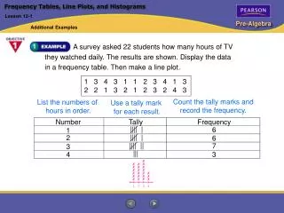
Count the tally marks and record the frequency. List the numbers of hours in order. Use a tally mark for each result. Number Tally Frequency 6 1 2 6 |||| | 7 3 |||| | ||| 4 3 |||| || Frequency Tables, Line Plots, and Histograms Lesson 12-1 Additional Examples A survey asked 22 students how many hours of TV they watched daily. The results are shown. Display the data in a frequency table. Then make a line plot. 1 3 4 3 1 1 2 3 4 1 3 2 2 1 3 2 1 2 3 2 4 3
“How many cases are you trying?” Number Frequency 0 3 1 5 2 4 3 5 4 4 Frequency Tables, Line Plots, and Histograms Lesson 12-1 Additional Examples Twenty-one judges were asked how many cases they were trying on Monday. The frequency table below shows their responses. Display the data in a line plot. Then find the range.
For a line plot, follow these steps 1 , 2 , and 3 . 3 Write a title that describes the data. Cases Tried by Judges x x x x x x x x x x x x x x x x x x x x x 2 Mark an x for each response. 0 1 2 3 4 1 Draw a number line with the choices below it. Frequency Tables, Line Plots, and Histograms Lesson 12-1 Additional Examples (continued) The greatest value in the data set is 4 and the least value is 0. So the range is 4 – 0, or 4.
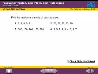
Step 1: Arrange the data in order from least to greatest. Find the median. 21 21 22 28 29 33 35 40 49 54 61 61 62 72 75 Step 2: Find the lower quartile and upper quartile, which are the medians of the lower and upper halves. 21 21 22 28 29 33 354049 54 61 61 62 72 75 lower quartile = 28 upper quartile = 61 Box-and-Whisker Plots Lesson 12-2 Additional Examples The data below represent the wingspans in centimeters of captured birds. Make a box-and-whisker plot. 61 35 61 22 33 29 40 62 21 49 72 75 28 21 54
Step 3: Draw a number line. Mark the least and greatest values, the median, and the quartiles. Draw a box from the first to the third quartiles. Mark the median with a vertical segment. Draw whiskers from the box to the least and greatest values. Box-and-Whisker Plots Lesson 12-2 Additional Examples (continued)
Draw a number line for both sets of data. Use the range of data points to choose a scale. Draw the second box-and-whisker plot below the first one. Box-and-Whisker Plots Lesson 12-2 Additional Examples Use box-and-whisker plots to compare test scores from two math classes. Class A: 92, 84, 76, 68, 90, 67, 82, 71, 79, 85, 79 Class B: 78, 93, 81, 98, 69, 95, 74, 87, 81, 75, 83
Box-and-Whisker Plots Lesson 12-2 Additional Examples Describe the data in the box-and-whisker plot. The lowest score is 55 and the highest is 85. One fourth of the scores are at or below 66 and one fourth of the scores are at or above 80. Half of the scores are at or between 66 and 80 and thus within 10 points of the median, 76.
Box-and-Whisker Plots Lesson 12-2 Additional Examples The plots below compare the percents of students who were eligible to those who participated in extracurricular activities in one school from 1992 to 2002. What conclusions can you draw? About 95% of the students were eligible to participate in extracurricular activities. Around 60% of the students did participate. A little less than two thirds of the eligible students participated in extracurricular activities.
Using Graphs to Persuade Lesson 12-3 Additional Examples Which title would be more appropriate for the graph below: “Texas Overwhelms California” or “Areas of California and Texas”? Explain.
Using Graphs to Persuade Lesson 12-3 Additional Examples (continued) Because of the break in the vertical axis, the bar for Texas appears to be more than six times the height of the bar for California. Actually, the area of Texas is about 267,000 mi2, which is not even two times the area of California, which is about 159,000 mi2. The title “Texas Overwhelms California” could be misleading. “Areas of Texas and California” better describes the information in the graph.
Using Graphs to Persuade Lesson 12-3 Additional Examples Study the graphs below. Which graph gives the impression of a sharper increase in rainfall from March to April? Explain.
Using Graphs to Persuade Lesson 12-3 Additional Examples (continued) In the second graph, the months are closer together and the rainfall amounts are farther apart than in the first graph. Thus the line appears to climb more rapidly from March to April in the second graph.
Using Graphs to Persuade Lesson 12-3 Additional Examples What makes the graph misleading? Explain. The “cake” on the right has much more than two times the area of the cake on the left.
mayonnaise Each branch of the “tree” represents one choice—for example, wheat-ham-mayonnaise. ham mustard wheat mayonnaise turkey mustard mayonnaise ham mustard white mayonnaise turkey mustard Counting Outcomes and Theoretical Probability Lesson 12-4 Additional Examples The school cafeteria sells sandwiches for which you can choose one item from each of the following categories: two breads (wheat or white), two meats (ham or turkey), and two condiments (mayonnaise or mustard). Draw a tree diagram to find the number of sandwich choices. There are 8 possible sandwich choices.
first digit, possible choices second digit, possible choices numbers, possible choices 5 • 5 = 25 Counting Outcomes and Theoretical Probability Lesson 12-4 Additional Examples How many two-digit numbers can be formed for which the first digit is odd and the second digit is even? There are 25 possible two-digit numbers in which the first digit is odd and the second digit is even.
right right wrong right wrong wrong number of favorable outcomes number of possible outcomes Use the probability formula. P(event) = 1 4 = 1 4 The probability of guessing correctly on two true/false questions is . Counting Outcomes and Theoretical Probability Lesson 12-4 Additional Examples Use a tree diagram to show the sample space for guessing right or wrong on two true-false questions. Then find the probability of guessing correctly on both questions. The tree diagram shows there are four possible outcomes, one of which is guessing correctly on both questions.
1st digit outcomes 10 2nd digit outcomes 10 3rd digit outcomes 10 4th digit outcomes 10 5th digit outcomes 10 total outcomes = 100,000 • • • • number of favorable outcomes number of possible outcomes P(winning number) = = 1 20,000 The probability is , or . 5 100,000 5 100,000 Counting Outcomes and Theoretical Probability Lesson 12-4 Additional Examples In some state lotteries, the winning number is made up of five digits chosen at random. Suppose a player buys 5 tickets with different numbers. What is the probability that the player has a winning number? First find the number of possible outcomes. For each digit, there are 10 possible outcomes, 0 through 9. Then find the probability when there are five favorable outcomes.
1 6 P(5) = There is one 5 among 6 numbers on a number cube. 3 6 P(less than 4) = There are three numbers less than 4 on a number cube. P(5, then less than 4) = P(5) • P(less than 4) 1 6 3 6 = • 3 36 1 12 1 12 = , or The probability of rolling 5 and then a number less than 4 is . Independent and Dependent Events Lesson 12-5 Additional Examples You roll a number cube once. Then you roll it again. What is the probability that you get 5 on the first roll and a number less than 4 on the second roll?
P(a seed grows) = 50%, or 0.50 Write the percent as a decimal. Substitute. = 0.50 • 0.50 Multiply. = 0.25 Write 0.25 as a percent. = 25% Independent and Dependent Events Lesson 12-5 Additional Examples Bluebonnets grow wild in the southwestern United States. Under the best conditions in the wild, each bluebonnet seed has a 20% probability of growing. Suppose you plant bluebonnet seeds in your garden and use a fertilizer that increases to 50% the probability that a seed will grow. If you select two seeds at random, what is the probability that both will grow in your garden? P(two seeds grow) = P(a seed grows) • P(a seed grows) The probability that two seeds will grow is 25%.
2 5 P(boy) = Two of five students are boys. If a boy’s name is drawn, one of the four remaining students is a boy. 1 4 P(boy after boy) = 2 5 1 4 Substitute. = • 2 20 1 10 1 10 Simplify. = , or The probability that both representatives will be boys is . Independent and Dependent Events Lesson 12-5 Additional Examples Three girls and two boys volunteer to represent their class at a school assembly. The teacher selects one name and then another from a bag containing the five students’ names. What is the probability that both representatives will be boys? P(boy, then boy) = P(boy) • P(boy after boy)
1st letter 5 choices 5 2nd letter 4 choices 4 3rd letter 3 choices 3 4th letter 2 choices 2 5th letter 1 choice 1 = 120 • • • • Permutations and Combinations Lesson 12-6 Additional Examples Find the number of permutations possible for the letters H, O, M, E, and S. There are 120 permutations of the letters H, O, M, E, and S.
7 studentsChoose 3. 7P3 Permutations and Combinations Lesson 12-6 Additional Examples In how many ways can you line up 3 students chosen from 7 students for a photograph? = 7 • 6 • 5 = 210 Simplify You can line up 3 students from 7 in 210 ways.
State Area (mi2) Alabama Colorado Maine Oregon Texas 50,750 103,729 30,865 96,003 261,914 Permutations and Combinations Lesson 12-6 Additional Examples In how many ways can you choose two states from the table when you write reports about the areas of states? Make an organized list of all the combinations.
Permutations and Combinations Lesson 12-6 Additional Examples (continued) AL, COAL, MEAL, ORAL, TXUse abbreviations of each CO, MECO, ORCO, TXstate’s name. First, list all ME, ORME, TXpairs containing Alabama. OR, TXContinue until every pair of states is listed. There are ten ways to choose two states from a list of five.
9 toppingsChoose 5. 9C5 9P5 5P5 = 9 • 81 • 7 • 62 • 51 51 • 41 • 31 • 21 • 1 = = 126 Simplify. Permutations and Combinations Lesson 12-6 Additional Examples How many different pizzas can you make if you can choose exactly 5 toppings from 9 that are available? You can make 126 different pizzas.
Permutations and Combinations Lesson 12-6 Additional Examples Tell which type of arrangement—permutations or combinations—each problem involves. Explain. a. How many different groups of three vegetables could you choose from six different vegetables? b. In how many different orders can you play 4 DVDs? Combinations; the order of the vegetables selected does not matter. Permutations; the order in which you play the DVDs matters.
P(event) = number of times an event occurs number of times an experiment is done = = 0.49 1,715 3,500 Experimental Probability Lesson 12-7 Additional Examples A medical study tests a new medicine on 3,500 people. It produces side effects for 1,715 people. Find the experimental probability that the medicine will cause side effects. The experimental probability that the medicine will cause side effects is 0.49, or 49%.
number of times an event occurs number of times an experiment is done Here are the results of 50 trials. 22431 13431 43121 21243 33434 32134 12224 42213 34424 32412 P(event) = = = The experimental probability of guessing correctly is . 10 50 1 5 1 5 Experimental Probability Lesson 12-7 Additional Examples Simulate the correct guessing of answers on a multiple-choice test where each problem has four answer choices (A, B, C, and D). Use a 4-section spinner to simulate each guess. Mark the sections as 1, 2, 3, and 4. Let “1” represent a correct choice.
Random Samples and Surveys Lesson 12-8 Additional Examples You want to find out how many people in the community use computers on a daily basis. Tell whether each survey plan describes a good sample. Explain. a. Interview every tenth person leaving a computer store. b. Interview people at random at the shopping center. c. Interview every tenth student who arrives at school on a school bus. This is not a good sample. People leaving a computer store are more likely to own computers. This is a good sample. It is selected at random from the population you want to study. This is not a good sample. This sample will be composed primarily of students, but the population you are investigating is the whole community.
defective sample calculators sample calculators defective calculators calculators Write a proportion. = 2 300 n 20,000 = Substitute. Write cross products. 2(20,000) = 300n 2(20,000) 300 300n 300 Divide each side by 300. = Simplify. 133 n Random Samples and Surveys Lesson 12-8 Additional Examples From 20,000 calculators produced, a manufacturer takes a random sample of 300 calculators. The sample has 2 defective calculators. Estimate the total number of defective calculators. Estimate: About 133 calculators are defective.
You can use a spinner to simulate the problem. Construct a spinner with seven congruent sections. Make five of the sections blue and two of them red. The blue sections represent not getting a base hit and the red sections represent getting a base hit. Each spin represents one time at bat. Problem Solving Strategy: Simulate the Problem Lesson 12-9 Additional Examples A softball player has an average of getting a base hit 2 times in every 7 times at bat. What is an experimental probability that she will get a base hit the next time she is at bat?
B B B BR RB BRB BRB BRB B B BR RB BRB B B BRB B B B B B B B B B B B BRB B BRB B B B B BR RB B B BR RB B B B B B B B B B B B B B BR RB B BR RB BRB B B B B B B B BRB B BR Problem Solving Strategy: Simulate the Problem Lesson 12-9 Additional Examples (continued) Use the results given in the table below. “B” stands for blue and “R” stands for red.
Makes a Base Hit Doesn’t Make a Base Hit |||| |||| |||| |||| || |||| |||| |||| |||| |||| |||| |||| |||| |||| |||| |||| |||| |||| |||| |||| ||| Problem Solving Strategy: Simulate the Problem Lesson 12-9 Additional Examples (continued) Make a frequency table. An experimental probability that she gets a base hit the next time she is at bat is 0.22, or 22%.