Chapter 10 Section 1: Scatter Diagrams & Linear Correlation
500 likes | 852 Vues
Chapter 10 Section 1: Scatter Diagrams & Linear Correlation. Created by: Mrs. Lowery. Scatter Diagram. X & Y Plot X – Explanatory Variable Y – Response Variable Looking for a Linear Relationship. Lab. Heart Rate Hours exercise per week. Line of “Best-fit”.

Chapter 10 Section 1: Scatter Diagrams & Linear Correlation
E N D
Presentation Transcript
Chapter 10 Section 1: Scatter Diagrams & Linear Correlation Created by: Mrs. Lowery
Scatter Diagram • X & Y Plot • X – Explanatory Variable • Y – Response Variable • Looking for a Linear Relationship
Lab • Heart Rate • Hours exercise per week
Line of “Best-fit” • 1 line the best-fits the points of the scatter diagram • More coming soon!
Correlation (r) • Perfect Linear • Positive (little x with little y & big x with big y) • Negative (little x with big y & big x with little y) • No Correlation • NO UNIT MEASURE
Cautions about Correlation • r = SAMPLE correlation coefficient computed from SAMPLE DATA • p (row) = Population correlation coefficient computed from ALL population data pairs • Correlation coefficient is a mathematical tool for measuring the strength of a linear relationship between 2 variables – No CAUSE AND EFFECT
Continued…. • NO CAUSE AND EFFECT • Lurking variables – it is neither part of the explanatory (x) or response (y) , but may be responsible for changes in both x and y.
Technology • Calculator – • Go the Catalog and turn Diagnostics On • Stat – Calc – 8: LinReg(a+bx) • Minitab • Stat- Basic Statistics - Correlation
Ch10 Sec 2: Linear Regression & Coefficient of Regression Created by: Mrs. Lowery
“Best” Linear Equation • Least-Square Criterion • Sum of the squares of the vertical distances from the data points (x,y) to the line is made as small as possible • See pg 603
Least Square Line • - estimate • a = y-intercept • b = slope • How many units the response variable is expected to change for each unit change in the explanatory variable (Marginal Change)
How To • b is with the x because in stats only 1 explanatory variable • See AP Formula Packet
Application • Making predictions • How Good of a prediction? - r
Problems • Interpolation • Predicting values between observed x values. • Extrapolation • Predicting values beyond the observed x values. • Do not do this • Height example • Note – there are confidence intervals for predictions • Note – You can only predict y from x not the other way around using this equation!
Technology • Calculator • Input data in lists • Stat – calc – 8:LinReg(a+bx) • Y= - vars – 5:Statistics – EQ – 1:RegEQ • Turn on Stat Plot • Zoom – 9:ZoomStat
Technology • Minitab • Input data • Stat – Regression – Fitted Line Plot
Coefficient of Determination • Answers: How good is the line as a instrument of regression? • The square of the sample correlation coefficient r
- Coefficient of Determination Total Deviation Explained Deviation Unexplained Deviation
Meaning of • ___ % of the (variation) behavior of the y variable can be explained by the corresponding (variation) behavior of the x variable if we use the least-square equation ________. • The remaining variation 1- __ = due to chance or lurking variables.
Ch10 Sec 3: Inferences for Correlation and Regression Created by: Mrs. Lowery
Musts to make inferences for population! • (x,y) are all random samples from the entire population • x and y are normally distributed • Variances are approximately equal • Their means lie on the least-square line
Hypothesis Testing: • Null – no correlation • Alternative • Set alpha level (.1, .05, .01)
Converting r into t-test n = number of sample data pairs Find p-value!
Interpretation • Reject Null • Fail to Reject Null • State your conclusion is context! • Remember NO CAUSE AND EFFECT
3 Measures of Scatter Diagram Spread: • Coefficient of Correlation • Coefficient of Determination • Standard Error of Estimate AND
Interpretation of SE • 0 = points all on line • Low value means --- Data points close • Higher values mean --- More Scattered
How to Find SE • Obtain a random sample of more than 3 pairs • Find the equation • Computation Formula for Standard Error of Estimate: (do not round too much)
Technology • Calculator • Put data in lists • Stat-Test-E:LinRegTTest • Minitab • Stat-Regression-Regression • The value of the standard error is displayed as s.
Confidence Interval • Sample = error • How to Calculate • Obtain sample of 3 or more • Find
More How To: • Find c – confidence interval for y for a specified x • c = Confidence Level (0 < c < 1) • n = Number of data pairs (at least 3) • = Critical value using d.f.=n - 2 • = Standard error of estimate
Interpret Confidence Interval I am ___% sure that the interval between ___ and ___ is one that contains the predicted amount of _________ that will _______ at (x-value).
Note: Confidence Band • The closer the interval is to the sample mean the tighter the confidence interval • Another reason for not extrapolating data.
Technology • Minitab – • Stat – Regression – Regression • Options • Enter observed x • Set Confidence Level • In Output – see %PI
Confidence Interval for Population Slope d.f.= n-2 Standard Error for b
How To: • State Null • State Alternative • State Confidence Level • Find test statistic • d.f = n-2 • Find the corresponding p-value • Conclusion • Context
Confidence Interval for • c = Confidence Level (0 < c < 1) • n = Number of data pairs (at least 3) • = Critical value using d.f.=n - 2 • = Standard error of estimate
Technology • Calculator • Stat • Test • E:LinRegTTest • Note: s – is standard error of measurement • Minitab • Stat • Regression • Regression • Note: s – is standard error of measurement • Gives results as 2-tailed – if 1-tailed divide p by 2
Ch10 Sec 4: Multiple Regression Created by: Mrs. Lowery
Multiple Regression • Predict “y” based on more than 1 x Response Variable Explanatory Variable(s) Coefficients from Least-square Regression We will only calculate using Minitab!
Regression Model • Identify Variables • One Response • All others = Explanatory • Collect Data for all variables • Find Equation • Check “goodness of fit” • Use Equation for prediction • Construct Confidence Intervals
How To: • Find Summary Statistics for each variable • Stat – Basic Statistic – Display Descriptive Statistic • Find correlation between variables • Stat – Basic Statistic – Correlation • Looking for r close to 1 thus more explained variability • Least – square equation • Choose 1 response variable • The rest are explanatory • Stat – regression – regression • In dialogues box select Response Variable • All other variables in other area
How well does our equation fit? • Examine coefficient of multiple determination • R-Sq = ___ % • % is the amount of explained variation that can be explained by the equation ____ and the joint variables (explanatory variables) together.
Prediction • Stat – Regression – Regression • Options: • List new observations (explanatory variables) • Check fit intercept • Value predicted for response variable • The output %PI - % Confidence Interval for Prediction • A confidence interval for a sample
Testing a Coefficient for Significance • Is every explanatory variable necessary??? Explanatory variable DOES Contribute Explanatory variable does NOT contribute
Interpret • Reject Null • Keep variable • Fail to Reject Null • Get Rid of Variable
Confidence interval for Coefficients Degrees of Freedom = n – k - 1 Coefficient t-critical from chart Standard Error/Deviation