Well Log Data Inversion Using Radial Basis Function Network
This paper presents innovative techniques for well log data inversion utilizing modified two-layer and proposed three-layer Radial Basis Function (RBF) networks. We explore the limitations of traditional methods and demonstrate the effectiveness of our models through simulations with real well log data. Our approach includes the implementation of K-means clustering for optimal node selection and the Generalized delta learning rule for weight adjustments. Results highlight improvements in layer effect accuracy, offering valuable insights into true formation conductivity from apparent conductivity measurements.

Well Log Data Inversion Using Radial Basis Function Network
E N D
Presentation Transcript
Well Log Data Inversion Using Radial Basis Function Network Kou-Yuan Huang,Li-Sheng Weng Department of Computer Science National Chiao Tung University Hsinchu, Taiwan kyhuang@cs.nctu.edu.tw and Liang-Chi Shen Department of Electrical & Computer Engineering University of Houston Houston, TX
Outline • Introduction • Proposed Methods • Modification of two-layer RBF • Proposed three-layer RBF • Experiments • Simulation using two-layer RBF • Simulation using three-layer RBF • Application to real well log data inversion • Conclusions and Discussion
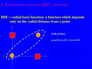
Review of well log data inversion • Lin, Gianzero, and Strickland used the least squares technique, 1984. • Dyos used maximum entropy, 1987. • Martin, Chen, Hagiwara, Strickland, Gianzero, and Hagan used 2-layer neural network, 2001. • Goswami, Mydur, Wu, and Hwliot used a robust technique,2004. • Huang, Shen, and Chen used higher order perceptron, IEEE IGARSS, 2008.
Review of RBF • Powell, 1985, proposed RBF for multivariate interpolation. • Hush and Horne, 1993,used RBF network for functional approximation. • Haykin, 2009, summarized RBF in Neural Networks book.
Properties of RBF • RBF is a supervised training model. • The 1st layer used the K-means clustering algorithm todetermine the K nodes. • The activation function of the 2nd layer was linear. f(s)=s. f ’(s)=1. • The 2ndlayer used the Widrow-Hoff learning rule.
Output of the 1st layer of RBF • Get mean & variance of each cluster from K-means clustering algorithm. • Cluster number K is pre-assigned. • Variance • Output of the 1st layer: response of Gaussian basis function
Training in the 2nd layer • Widrow-Hoff’s learning rule. • Error function • Use gradient descent method to adjust weights f(s)=s. =1
Outline • Introduction • Proposed Methods • Modification of two-layer RBF • Proposed three-layer RBF • Experiments • Simulation using two-layer RBF • Simulation using three-layer RBF • Application to real well log data inversion • Conclusions and Discussion
Optimal number of nodes in the 1st layer • We use K-means clustering algorithm & Pseudo F-Statistics (PFS) (Vogel and Wong, 1979) to determine the optimal number of nodes in the 1st layer. • PFS: n is the pattern number. K is the cluster number. • Select K when PFS is the maximum. Kbecomes the node number in the 1st layer.
Perceptron training in the 2nd layer • Activation function at the 2nd layer: sigmoidal • Error Function • Delta learning rule(Rumelhart, Hinton, and Williams, 1986): use gradient descent method to adjust weights
Outline • Introduction • Proposed Methods • Modification of two-layer RBF • Proposed three-layer RBF • Experiments • Simulation using two-layer RBF • Simulation using three-layer RBF • Application to real well log data inversion • Conclusions and Discussion
Generalized delta learning rule (Rumelhart, Hinton, and Williams, 1986) • Adjust weights between the 2nd layer and the 3rd layer • Adjust weights between the 1st layer and the 2nd layer, • Adjust weights with momentum term:
Outline • Introduction • Proposed Methods • Modification of two-layer RBF • Proposed three-layer RBF • Experiments • Simulation using two-layer RBF • Simulation using three-layer RBF • Application to real well log data inversion • Conclusions and Discussion
Experiments: System flow in simulation True formationresistivity(Rt) Apparent resistivity (Ra) Apparent conductivity (Ca) Re-scale Ct’ to Ct Radial basis function network (RBF) Scale Ca to 0~1 (Ca’) True formation conductivity (Ct’) Desired true formationconductivity (Ct’’)
Experiments: on simulated well log data • In the simulation, there are 31 well logs. • Professor Shenat University of Houston worked on theoretical calculation. • Each well log has the apparent conductivity (Ca) as the input, and the true formation conductivity (Ct) as the desired output. • Well logs #1~#25 are for training. • Well logs #26~#31 are for testing.
Simulated well log data: examples • Simulated well log data #7
What is the input data length? Output length? • 200 records on each well log. 25 well logs for training. 6 well logs for testing. • How many inputs to the RBF is the best? Cut 200 records into 1, 2, 4, 5, 10, 20, 40, 50, 100, and 200 data, segment by segment, to test the best input data length to RBF model. • For inversion, the output data length is equal to the input data length in the RBF model. • In testing, input n data to the RBF model to get the n output data, then input n data of the next segment to get the next n output data, repeatedly.
Example of input data lengthat well log #13 • If each segment (pattern vector) has 10 data, 200 records of each well log are cut into 20 segments (pattern vectors).
Input data length and # of training patterns from 25 training well logs
Optimal cluster number of training patternsExample: for input data length 10 • PFS vs. K. For input N=10, the optimal cluster number K is 27.
Optimal cluster number of training patterns in 10 cases • Set up 10 two-layer RBF models. • Compare the testing errors of 10 models to select the optimal RBF model.
Parameter setting in the experiment • Parameters in RBF training Learning rate : 0.6 Momentum coefficient : 0.4 (in 3-layer RBF) Maximum iterations: 20,000 Error threshold: 0.002. • Define mean absolute error (MAE): Pis the pattern number, K is the output nodes.
Testing errors at 2-layer RBF models in simulation • 10-27-10 RBF model gets the smallest error in testing.
Training result: error vs. iterationusing 10-27-10 two-layer RBF
Inversion testing using 10-27-10 two-layer RBF • Inverted Ct of log #27 by network 10-27-10 (MAE= 0.055537). • Inverted Ct of log #26 by network 10-27-10 (MAE= 0.051753).
Inverted Ct of log #28 by network 10-27-10 (MAE= 0.041952). • Inverted Ct of log #29 by network 10-27-10 (MAE= 0.040859).
Inverted Ct of log #31 by network 10-27-10 (MAE= 0.050294). • Inverted Ct of log #30 by network 10-27-10 (MAE= 0.047587).
Outline • Introduction • Proposed Methods • Modification of two-layer RBF • Proposed three-layer RBF • Experiments • Simulation using two-layer RBF • Simulation using three-layer RBF • Application to real well log data inversion • Conclusions and Discussion
Experiment: Training in modified three-layer RBF.Hidden node number?
Determine the number of hidden nodes in the 2-layer perceptron • On hidden nodes for neural nets (Mirchandani and Cao,1989) It divides space to maximum M regions when input space is d dimensions and there are H hidden nodes. T: number of training patterns. Each pattern is in one region. From T ≈ M, we can determine H hidden nodes.
Hidden node number and optimal 3-layer RBF • 10-27-10 2-layer RBF gets the smallest error in testing. We extend it to 10-27-H-10 in the 3-layer RBF. H=? • For original 10 inputs, the number of training patterns is 500. T=500. • For a 27-H-10 two-layer perceptron, the number of input nodes is 27. When d=27, H=9 (=500), we select hidden node number H=9. • Finally, we get 10-27-9-10 as the optimal 3-layer RBF model.
Training result: error vs. iterationusing 10-27-9-10 three-layer RBF
Inversion testing using 10-27-9-10 three-layer RBF • Inverted Ct of log 26 by network 10-27-9-10 (MAE= 0.041526) • Inverted Ct of log 27 by network 10-27-9-10 (MAE= 0.059158)
Inverted Ct of log 28 by network 10-27-9-10 (MAE= 0.046744) • Inverted Ct of log 29 by network 10-27-9-10 (MAE= 0.043017)
Inverted Ct of log 30 by network 10-27-9-10 (MAE= 0.046546) • Inverted Ct of log 31 by network 10-27-9-10 (MAE= 0.042763)
Testing error of each well log using 10-27-9-10 three-layer RBF model Average error: 0.046625
Average testing error of each three-layer RBF model in simulation • Experiments using RBFs with different number of hidden nodes. • 10-27-9-10 get the smallest average error in testing. So it is selected to the real data application.
Outline • Introduction • Proposed Methods • Modification of two-layer RBF • Proposed three-layer RBF • Experiments • Simulation using two-layer RBF • Simulation using three-layer RBF • Application to real well log data inversion • Conclusions and Discussion