Linear Programming Interior-Point Methods
Linear Programming Interior-Point Methods. D. Eiland. Linear Programming Problem. LP is the optimization of a linear equation that is subject to a set of constraints and is normally expressed in the following form :. Minimize :. Subject to :. Barrier Function.

Linear Programming Interior-Point Methods
E N D
Presentation Transcript
Linear ProgrammingInterior-Point Methods D. Eiland
Linear Programming Problem LP is the optimization of a linear equation that is subject to a set of constraints and is normally expressed in the following form : Minimize : Subject to :
Barrier Function To enforce the inequality on the previous problem, a penalty function can be added to Then if any xj 0, then trends toward As , then is equivalent to
Lagrange Multiplier To enforce the constraints, a Lagrange Multiplier (-y) can be added to Giving a linear function that can be minimized.
Optimal Conditions Previously, we found that the optimal solution of a function is located where its gradient (set of partial derivatives) is zero. That implies that the optimal solution for L(x,y) is found when : Where :
Optimal Conditions (Con’t) By defining the vector , the previous set of optimal conditions can be re-written as
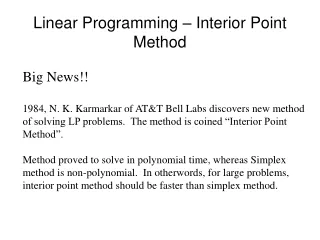
Newton’s Method Newton’s method defines an iterative mechanism for finding a function’s roots and is represented by : When ,
Optimal Solution Applying this to we can derive the following :
Interior Point Algorithm This system can then be re-written as three separate equations : Which is used as the basis for the interior point algorithm : • Choose initial points for x0,y0,z0 and the select value for τ between 0 and 1 • While Ax - b != 0 • Solve first above equation for Δy [Generally done by matrix factorization] • Compute Δx and Δz • Determine the maximum values for xn+1, yn+1,zn+1 that do not violate the constraints x >= 0 and z >= 0 from : With : 0 < a <=1