Download

1 / 55
560 likes | 1.08k Vues
Even though both statistics centered at the parameter value, the probability that A is closer to the parameter value is higher than the probability that B is closer to the parameter value.

E N D
Even though both statistics centered at the parameter value, the probability that A is closer to the parameter value is higher than the probability that B is closer to the parameter value. • It is better to use a statistics which is centered at the parameter and has smaller variation, i.e. smaller standard error.
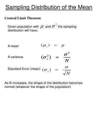
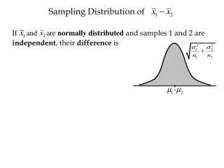
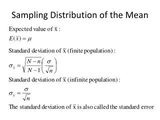
Standard deviation of the sampling distribution equals That is, Properties of the Sampling Distribution of x • Mean of the sampling distribution equals mean of sampled population*, that is, Standard error of sample mean
Theorem 5.1 If a random sample of n observations is selected from a population with a normal distribution, the sampling distribution of will be a normal distribution.
s = 10 m = 50 x Sampling from Normal Populations • Central Tendency • Dispersion • Sampling with replacement Population Distribution Sampling Distribution n = 4x = 5 n =16x= 2.5 m - = 50 x x
Sampling Distribution Standardized Normal Distribution s s = 1 x m m = 0 z x x Standardizing the Sampling Distribution of x
Sampling from Non-Normal Populations • Central Tendency • Dispersion • Sampling with replacement Population Distribution s = 10 m = 50 x Sampling Distribution n = 4x= 5 n =30x = 1.8 m - = 50 x x
Central Limit Theorem Consider a random sample of n observations selected from a population (any probability distribution) with mean μ and standard deviation . Then, when n is sufficiently large, the sampling distribution of will be approximately a normal distribution with mean and standard deviation The larger the sample size, the better will be the normal approximation to the sampling distribution of .
sampling distribution becomes almost normal. Central Limit Theorem As sample size gets large enough (n 30) ... x
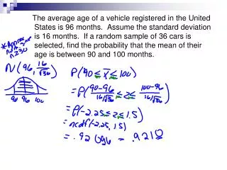
Thinking Challenge • Assume that the systolic blood pressure of 30-year-old males is normally distributed, with an average of 122 mmHg and a standard deviation of 10mmHg. A random sample of 16 men from this age group is selected. • Calculate the probability that the average blood pressure of the sample will be greater than 125mmHg? • Calculate the probability that the average blood pressure of this sample will be between 118 and 124 mmHg? • Calculate the probability that the blood pressure of an individual male from this population will be between 118 and 124mmHg?
Thinking Challenge • Assume that the average weight of an NFL player is 245.7 pounds with a standard deviation of 34.5 pounds, but the probability distribution of the population is unknown. If a random sample of 32 players is selected, • what is the probability that the average weight of the sample will be less than 234 pounds? • What is the probability that the average weight of the sample is between 248 and 254 pounds?
The Sampling Distribution of the Sample Proportion (Predicting the behavior of discrete random variables)
Sample Proportion Just as the sample mean is a good estimator of the population mean, the sample proportion—denoted — is a good estimator of the population proportion p. How good the estimator is will depend on the sampling distribution of the statistic. This sampling distribution has properties similar to those of the sampling distribution of
Thinking Challenge • A report claims that 15% of women are left-handed. a) Calculate the probability that more than 12% of a random sample of 100 women is left-handed. np=100*0.15=15≥15 n(1-p)=100*0.85=85 ≥15 So we can use the normal approximation to the binomial distribution.
Thinking Challenge (cont.) b) Calculate the probability that 11% to 16%-women random sample is left-handed.
6.4 Largesampleconfidenceintervalforproportion
Example • Coral reef communities are home to one quarter of all marine plants and animals world wide. • These reefs are very important. • They suport large fisheries. • They protect shorelines against tides, storm surges, and hurricanes. • Marine scientists say that pollution, global warming, and increasind acidification of the oceans destroy reef systems.
Example (cont.) • A group of scientists study corals and the diseases that affect them. • They sampled sea fans at 19 randomly selected reefs along the Yucatan peninsula and diagnosed whether the animals were affected by the specific disease. • In specimens collected at a depth of 40 feet at the Las Redes Reef in Akumal, Mexico, these scientists found that 54 of 104 sea fans sampled were infected with that disease.
Example (cont.) • Of course we care about the much more than these particular 104 sea fans. • We care about the health of coral reef communities throughout the Caribbean. • What can this study tell us about that?
Example (cont.) • We have a sample proportion of 51.9%. • Our first guess might be that this observed proportion is close to the population proportion. • But because of the sampling variability, if the researchers had drawn a second sample of 104 sea fans at roughly same time, the proportion for the infected wouldn’t have been exactly 51.9%. • What can we say about the population proportion, p?
Example (cont.) • To start to answer this question, we should think about how different the sample proportion might have been if we’d taken another random sample from the same population. • We are not actually going to take more samples. • We just want to imagine how the sample proportions might vary from sample to sample. • We want to know about the sampling distribution of the sample proportion of infected sea fans.
Example (cont.) • 2SE=0.098 • 3SE=0.147
Example (cont.) • By the 68-95-99.7% Rule, we know • about 68% of all samples of 104 seafans will have ’s within 1 SE, 0.049, of p • about 95% of all samples of 104 seafanswill have ’s within 2 SEs, 0.098, of p • about 99.7% of all samples of 104 seafanswill have ’s within 3 SEs, 0.147, of p • But where is oursampleproportion in thispicture? • Whatvaluedoesphave?
Example (cont.) • Weknowthatfor 95% of randomsamples, will be no morethan 2 SEsawayfrom p. • If I am , there is a 95% chancethat p is no morethan 2SEs awayfromme. • So, if Ireach out 2 SEs, I am95% sure that p will bewithinmygrasp. • Now, I’vegothim! Probably. • Of course, evenifmyintervalcatch p, I stilldon’tknowitstruevalue. • Thebest I can do is an interval, andeventhen I can’t be positive it contains p.
Confidence Interval • “We are 95% confident that between 42.1% and 61.7% of sea fans are infected.” • Statements like these are called confidence intervals.
What Does “95% Confidence” Really Mean? • Each confidence interval uses a sample statistic to estimate a population parameter. • But, since samples vary, the statistics we use, and thus the confidence intervals we construct, vary as well.
What Does “95% Confidence” Really Mean? (cont.) • The figure to the right shows that some of our confidence intervals (from 20 random samples) capture the true proportion (the green horizontal line), while others do not:
What Does “95% Confidence” Really Mean? (cont.) • Our confidence is in the process of constructing the interval, not in any one interval itself. • Thus, we expect 95% of all confidence intervals to contain the true parameter that they are estimating.
Margin of Error: Certainty vs. Precision • We can claim, with 95% confidence, that the interval contains the true population proportion. • The extent of the interval on either side of is called the margin of error (ME). • In general, confidence intervals have the form estimate± ME.
Whatifwewantedto be moreconfident? • To be moreconfident, we’llneedtocapture p moreoftenandto do thatwe’llneedtomaketheintervalwider. • The more confident we want to be, the larger our ME needs to be (makes the interval wider).
Margin of Error: Certainty vs. Precision (cont.) • To be more confident, we wind up being less precise. • Because of this, every confidence interval is a balance between certainty and precision. • The tension between certainty and precision is always there. • Fortunately, in most cases we can be both sufficiently certain and sufficiently precise to make useful statements. • To get a narrower interval without giving up confidence, you need to have less variability. • You can do this with a larger sample…
Margin of Error: Certainty vs. Precision (cont.) • The choice of confidence level is somewhat arbitrary, but keep in mind this tension between certainty and precision when selecting your confidence level. • The most commonly chosen confidence levels are 90%, 95%, and 99% (but any percentage can be used).
Critical Values • The ‘2’ in (our 95% confidence interval) came from the 68-95-99.7% Rule. • Using a table or technology, we find that a more exact value for our 95% confidence interval is 1.96 instead of 2. • We call 1.96 the critical value and denote it z*. • For any confidence level, we can find the corresponding critical value.
Critical Values (cont.) • Example: For a 90% confidence interval, the critical value is 1.645:
Assumptions and Conditions • All statistical models depend upon assumptions. • Different models depend upon different assumptions. • If those assumptions are not true, the model might be inappropriate and our conclusions based on it may be wrong. • You can never be sure that an assumption is true, but you can often decide whether an assumption is plausible by checking a related condition.
Assumptions and Conditions (cont.) • Here are the assumptions and the corresponding conditions you must check before creating a confidence interval for a proportion: • Independence Assumption: We first need to Think about whether the Independence Assumption is plausible. It’s not one you can check by looking at the data. Instead, we check randomization condition to decide whether independence is reasonable.
Assumptions and Conditions (cont.) • Randomization Condition: Were the data sampled at random or generated from a properly randomized experiment? Proper randomization can help ensure independence. • Sample Size Assumption: The sample needs to be large enough for us to be able to use the CLT. • Success/Failure Condition: We must expect at least 15 “successes” and at least 15 “failures.”
One-Proportion z-Interval • When the conditions are met, we are ready to find the confidence interval for the population proportion, p. • The confidence interval is where • The critical value, z*, depends on the particular confidence level, C, that you specify.
Thinking Challenge Plausibleindependence condition: It is reasonabletothinkthattheresponsesweremutuallyindependent, providedgoodsurveyingtechniqueswereused. Randomsampling condition: Thevotersweresampledrandomly. Sample size condition: 144 and 186 arebothlargerthan 15 sothesample is largeenough.
Thinking Challenge (cont.) Weare 95% confidentthatbetween 38.% and 49% of voterswillvote “yes” on theupcomingbudget.
Caution!!! • Unlessn is extremelylarge, thelargesampleprocedureperformspoorlywhen p is near 0 ornear 1. • Forinstance ; p= 0.001 and n=100 sothatnp=0.1 <15 • Unlesswehave an extremelylarge n we can not satisfythesample size assumption. • However, makingminoradjustment on thesampleproportion can handlethat problem.
Adjusted (1 – )100% Confidence Interval for a Population Proportion, p the adjusted sample proportion of observations with the characteristic of interest, x is the number of successes in the sample, and n is the sample size.
Example • AccordingtotheBureau of Labor Statistics (2012), theprobability of injurywhileworking at a jewelrystore is lessthan 0.01. Supposethat in a randomsample of 200 jewelrystoreworkers, 3 wereinjured on thejob. Estimatethetrueproportion of jewelrystoreworkerswhoareinjured on thejobusing 95% confidenceinterval.