Frequency Characteristics of AC Circuits
400 likes | 906 Vues
Chapter 17. Frequency Characteristics of AC Circuits. Introduction A High-Pass RC Network A Low-Pass RC Network A Low-Pass RL Network A High-Pass RL Network A Comparison of RC and RL Networks Bode Diagrams Combining the Effects of Several Stages RLC Circuits and Resonance

Frequency Characteristics of AC Circuits
E N D
Presentation Transcript
Chapter 17 Frequency Characteristics of AC Circuits • Introduction • A High-Pass RC Network • A Low-Pass RC Network • A Low-Pass RL Network • A High-Pass RL Network • A Comparison of RC and RL Networks • Bode Diagrams • Combining the Effects of Several Stages • RLC Circuits and Resonance • Filters • Stray Capacitance and Inductance
17.1 Introduction • Earlier we looked at the bandwidth and frequency response of amplifiers • Having now looked at the AC behaviour of components we can consider these in more detail • The reactance of both inductors and capacitance is frequency dependent and we know that
We will start by considering very simple circuits • Consider the potential divider shown here • from our earlier consideration of the circuit • rearranging, the gain of the circuit is • this is also called the transfer function of the circuit
17.2 A High-Pass RC Network • Consider the following circuit • which is shown re-drawn in a more usual form
Clearly the transfer function is • At high frequencies • is large, voltage gain 1 • At low frequencies • is small, voltage gain 0
Since the denominator has real and imaginary parts, the magnitude of the voltage gain is • When 1/CR = 1 • This is a halving of power, or a fall in gain of 3 dB
The half power point is the cut-off frequency of the circuit • the angular frequency C at which this occurs is given by • where is the time constant of the CR network. Also
Substituting =2f and CR = 1/ 2fC in the earlier equation gives • This is the general form of the gain of the circuit • It is clear that both the magnitude of the gain and the phase angle vary with frequency
Consider the behaviour of the circuit at different frequencies: • When f >> fc • fc/f << 1, the voltage gain 1 • When f = fc • When f << fc
The behaviour in these three regions can be illustrated using phasor diagrams • At low frequencies the gain is linearly related to frequency. It falls at -6dB/octave (-20dB/decade)
Frequency response of the high-pass network • the gain response hastwo asymptotes thatmeet at the cut-offfrequency • figures of this form are called Bode diagrams
17.3 A Low-Pass RC Network • Transposing the C and R gives • At high frequencies • is large, voltage gain 0 • At low frequencies • is small, voltage gain 1
17.3 A Low-Pass RC Network • A similar analysis to before gives • Therefore when, when CR = 1 • Which is the cut-off frequency
Therefore • the angular frequency C at which this occurs is given by • where is the time constant of the CR network, and as before
Substituting =2f and CR = 1/ 2fC in the earlier equation gives • This is similar, but not the same, as the transfer function for the high-pass network
Consider the behaviour of this circuit at different frequencies: • When f << fc • f/fc<< 1, the voltage gain 1 • When f = fc • When f >> fc
The behaviour in these three regions can again be illustrated using phasor diagrams • At high frequencies the gain is linearly related to frequency. It falls at 6dB/octave (20dB/decade)
Frequency response of the low-pass network • the gain response hastwo asymptotes thatmeet at the cut-offfrequency • you might like to compare this with the Bode Diagram for a high-pass network
17.4 A Low-Pass RL Network • Low-pass networks can alsobe produced using RL circuits • these behave similarly to thecorresponding CR circuit • the voltage gain is • the cut-off frequency is
17.5 A High-Pass RL Network • High-pass networks can alsobe produced using RL circuits • these behave similarly to thecorresponding CR circuit • the voltage gain is • the cut-off frequency is
17.6 A Comparison of RC and RL Networks • Circuits using RC and RLtechniques have similarcharacteristics • for a more detailedcomparison, seeFigure 17.10 in thecourse text
17.7 Bode Diagrams • Straight-line approximations
17.8 Combining the Effects of Several Stages • The effects of several stages ‘add’ in bode diagrams
Multiple high- and low-passelements may also be combined • this is illustrated in Figure 17.14in the course text
17.9 RLC Circuits and Resonance • Series RLC circuits • the impedance is given by • if the magnitude of the reactanceof the inductor and capacitor areequal, the imaginary part is zero,and the impedance is simply R • this occurs when
This situation is referred to as resonance • the frequency at which is occurs is the resonant frequency • in the series resonant circuit, the impedance is at a minimum at resonance • the current is at a maximum at resonance
The resonant effect can be quantified by the quality factor, Q • this is the ratio of the energy dissipated to the energy stored in each cycle • it can be shown that • and
The series RLC circuit is an acceptor circuit • the narrowness of bandwidth is determined by the Q • combining this equation with the earlier one gives
Parallel RLC circuits • as before
The parallel arrangement is a rejector circuit • in the parallel resonant circuit, the impedance is at a maximum at resonance • the current is at a minimum at resonance • in this circuit
17.10 Filters • RC Filters • The RC networks considered earlier are first-order or single-pole filters • these have a maximum roll-off of 6 dB/octave • they also produce a maximum of 90 phase shift • Combining multiple stages can produce filters with a greater ultimate roll-off rates (12 dB, 18 dB, etc.) but such filters have a very soft ‘knee’
An ideal filter would have constant gain and zero phase shift for frequencies within its pass band, and zero gain for frequencies outside this range (its stop band) • Real filters do not have theseidealised characteristics
LC Filters • Simple LC filters can be produced using series or parallel tuned circuits • these produce narrow-band filters with a centre frequency fo
Active filters • combining an op-amp with suitable resistors and capacitors can produce a range of filter characteristics • these are termed active filters
Common forms include: • Butterworth • optimised for a flat response • Chebyshev • optimised for a sharp ‘knee’ • Bessel • optimised for its phase response see Section 17.10.3 of the course text for more information on these
17.11 Stray Capacitance and Inductance • All circuits have stray capacitance and stray inductance • these unintended elements can dramatically affect circuit operation • for example: • (a) Cs adds an unintended low-pass filter • (b) Ls adds an unintended low-pass filter • (c) Cs produces an unintended resonant circuit and can produce instability
Key Points • The reactance of capacitors and inductors is dependent on frequency • Single RC or RL networks can produce an arrangement with a single upper or lower cut-off frequency. • In each case the angular cut-off frequency o is given by the reciprocal of the time constant • For an RC circuit = CR, for an RL circuit = L/R • Resonance occurs when the reactance of the capacitive element cancels that of the inductive element • Simple RC or RL networks represent single-pole filters • Active filters produce high performance without inductors • Stray capacitance and inductance are found in all circuits