Download
1 / 41
420 likes | 850 Vues
Lecture 14. X-Ray Fluorescence Microscopy. X-Ray Synchrotron. Giant x-ray ring located at Brookhaven National Laboratory in Long Island New York. Utilized soft x-ray microscopy to visualize chemical groups in paper. ESCA (XPS) with pictures. The Microscope.

E N D
Lecture 14. X-Ray Fluorescence Microscopy
X-Ray Synchrotron • Giant x-ray ring located at Brookhaven National Laboratory in Long Island New York. • Utilized soft x-ray microscopy to visualize chemical groups in paper. • ESCA (XPS) with pictures.
The Microscope • Scanning Transmission X-ray Microscope (STXM) • Operates between the K edges carbon and oxygen with good penetration in samples slightly less than 1μm, therefore well suited for the study of specimens like single biological cells. • Can operate under standard conditions or cryo conditions.
The Microscope (2) • Soft x-ray microscopy uses X rays with an energy of 100-1000 eV, or a wavelength of about 1-10 nm. X-ray energy (eV). • 30nm resolution • Only about 1 dozen sychrotron STXMs available worldwide.
Biological imaging • Consider penetration distance: 1/e absorption length for x rays, scattering mean free paths for electrons • Water window: Wolter, Ann. Phys.10, 94 (1952)
X rays Electrons • Inelastic scattering dominates (energy filters) • Multiple scattering often present • High contrast from small things • Absorption dominates • Inelastic scattering is weak • No multiple scattering
Thick samples: photons come out ahead X-rays: better for thicker specimens. Sayre et al., Science196, 1339 (1977) Schmahl & Rudolph (1990) These plots: Jacobsen, Medenwaldt, and Williams, in X-ray Microscopy & Spectromicroscopy (Springer, 1998)
Fibroblast reconstruction: Z slices Frozen-hydrated (ethane plunge) 3T3 fibroblast: Y. Wang et al., J. Microscopy197, 80 (2000)
Analyzing full fluorescence spectra • Peaks from trace elements can be on shoulders of strong peaks from common elements. • Setting simple energy windows can give poor quantitation. Record full spectrum and do curve-fitting! • Wavelength dispersive detectors can help – but often with lower collection solid angle • This example: Twining et al., Anal. Chem. 75, 3806 (2003). Also ESRF, elsewhere.
X-ray focusing: Fresnel zone plates Diameter d, outermost zone width drN, focal length f, wavelength : • Diffractive optics: radially varied grating spacing • Largest diffraction angle is given by outermost (finest) zone width drNas =/(2drN) • Rayleigh resolution is 0.61 /()=1.22drN • Zones must be positioned to ~1/3 width over diameter (10 nm in 100 m, or 1:104) Central stop and order sorting aperture (OSA) to isolate first order focus
Fresnel zone plate images R. W. Wood (1898): zone plate figure drawn with a pen and a compass! Photographically reduced
Zone plates by electron beam lithography • Electron beam lithography: produces the finest possible structures (other than what nature can be persuaded to make by itself). Many efforts worldwide! • M. Lu, A. Stein (PhD 2002; now BNL), S. Spector (PhD 1998; now Lincoln Lab), C. Jacobsen (Stony Brook) • D. Tennant (Lucent/New Jersey Nanotech Consortium) • JEOL JBX-9300FS: 1 nA into 4 nm spot, 1.2 nm over 500 m, 100 keV A. Stein and JBX-9300FS
TXM Incoherent illumination; works well with a bending magnet; exposure time of seconds More pixels (e.g., 20482) Moderate spectral resolution in most cases: E/(E)300-1000 STXM Coherent illumination; works best with an undulator; exposure time seconds to minutes Less dose to sample (~10% efficient ZP) Better suited to conventional grating monochromator: E/(E)3000-5000 Zone plate microscopes
Soft x-ray imaging NIL 8 fibroblast (glutaraldehyde fixed): V. Oehler, J. Fu, C. Jacobsen Human sperm (unfixed): S. Wirick, C. Jacobsen, Y. Shenkin Test pattern: see Jacobsen et al., Opt. Comm. 86, 351 (1991)
Immunogold labeling • H. Chapman, C. Jacobsen, and S. Williams, Ultramicroscopy62, 191 (1996). • Fibroblast, antibody labeled for tubulin. • More recent work: • C. Larabell et al., LBL/UCSF • S. Vogt et al., then at Göttingen • Labels must be comparable in size to optical resolution. Vogt and Jacobsen, Ultramicroscopy 87, 25 (2001) • Challenge: how to label without altering cell?
Absorption edges Lambert-Beer law: linear absorption coefficient µ This coefficient makes a jump at specific elemental absorption edges! This example: 0.1 µm protein, silica
X-ray microscopy of colloids • U. Neuhäusler (Stony Brook/Göttingen), S. Abend (Kiel), G. Lagaly (Kiel), C. Jacobsen (Stony Brook), Colloid and Polymer Science277, 719 (1999) • Emulsion: water, oil droplets, clay, and layered double hydroxides (LDH) • “Caged” part of oil droplet remains fixed; “uncaged” part can disperse 290 eV: carbon strongly absorbing 346 eV: calcium weakly absorbing. Clays and LDHs absorb equally 352.3 eV: calcium strongly absorbing. Calcium-rich LDHs are highlighted. 284 eV: carbon (oil drop) weakly absorbing
Near-edge absorption fine structure (NEXAFS) orX-ray absorption near-edge structure (XANES) • Fine-tuning of the x-ray energy near an atom’s edge gives sensitivity to the chemical bonding state of atoms of that type • First use in microscopy: Ade et al., Science 258, 972 (1992)
C-XANES of amino acids • K. Kaznacheyev et al., J. Phys. Chem. A 106, 3153 (2002) • Experiment: K. Kaznacheyev et al., Stony Brook (now CLS) • Theory: O. Plashkevych, H. Ågren et al., KTH Stockholm; A. Hitchcock, McMaster
Spectromicroscopy by image stacks • Acquire sequence of images over XANES spectral region; automatically align using Fourier cross-correlations or laser interferometer; extract spectra. • C. Jacobsen et al., J. Microscopy197, 173 (2000). Images at N=150 energies are common. Photon energy
DNA packing in sperm • X. Zhang, R. Balhorn, J. Mazrimas, and J. Kirz, J. Structural Biology116, 335 (1996) • DNA packing in sperm mediated by protamine I and protamine II; fraction of protamine II can vary from 0% to 67% among several species • Bulk measurements: compromised by immature or arrested spermatids • Images at six XANES resonance energies for each specimen
“Sperm morphology, motility, and concentration in fertile and infertile men” Guzick et al., New England Journal of Medicine345, 1388 (2001) “Although semen analysis is routinely used to evaluate the male partner in infertile couples, sperm measurements that discriminate between fertile and infertile men are not well defined… Threshold values for sperm concentration, motility, and morphology can be used to classify men as subfertile, of indeterminate fertility, or fertile. None of the measures, however, are diagnostic of infertility.”
What are the predictors of fertility? • Use chemical state mapping of x-ray microscopy to investigate sperm types from different patients (Holger Fleckenstein, Physics; Dr. Yefim Sheynkin, Dept. Urology) • Preparation: compare room temp wet (at right), frozen hydrated, freeze-dried • One in-vitro fertilization method: single sperm are selected for injection into egg. What’s the basis for choosing one sperm over another?
Cluster analysis of sperm Air-dried specimen; 140 separate images
Comparison with mitochondrial DNA spectrum Mitochondrial DNA spectrum: K. Kaznacheyev Mitochondrial DNA Purple region Purple region: DNA packed with protamines
Radiation damage on (initially) living cells Experiment by V. Oehler, J. Fu, S. Williams, and C. Jacobsen, Stony Brook using specimen holder developed by Jerry Pine and John Gilbert, CalTech • X-rays are ionizing radiation. The dose per high resolution image is about 100,000 times what is required to kill a person • Makes it hard to view living cells!
Wet, fixed samples: one image is OK • Chromosomes are among the most sensitive specimens. • V. faba chromosomes fixed in 2% glutaraldehyde. S. Williams et al., J. Microscopy170, 155 (1993) • Repeated imaging of one chromosome shows mass loss, shrinkage
Frozen hydrated specimens Grids with live cells are • Taken from culture medium and blotted • Plunged into liquid ethane (cooled by liquid nitrogen) • Loaded into cryo holder
Radiation damage resistance in cryo Maser et al., J. Microscopy197, 68 (2000) Left: frozen hydrated image after exposing several regions to ~1010 Gray Right: after warmup in microscope (eventually freeze-dried): holes indicate irradiated regions!
Lignocellulosics • Radicals are formed by the interaction of peroxide and metal that can damage cellulose • Damage results in carboxylic acid groups • Visualize the damage physical and chemical testing show H2O2 Mg H2O2 Mg
Sample Prep • Peroxide bleached and unbleached handsheets • Cut ~1cm by 2cm samples • Soaked in water • Dehydrated in ethanol • Used 50/50 mixture of epoxy resin (Epon 812) and propylene oxide • 100% epoxy and vacuum • Cured in oven between plastic sheets • Sectioned to 200nm thick (transverse) and placed on TEM grids
Locating Carboxylic Acids(unbleached) 285 289 TEM grid hole = ~125 μm
Locating Carboxylic Acids (2)(bleached) 285 289 TEM grid hole = ~125 μm
Locating Carboxylic Acids (3)(bleached) 285 289 TEM grid hole = ~125 μm
High Resolution(bleached) • Stepper scan (.5 μm) vs. piezo scan (30 nm). • High resolution images of damaged regions. • Perhaps evidence of hollow center. 285 289 285 289 Top = 20 μm Bottom = 8 μm
High Resolution (2)(unbleached) Left = 72 μm Right = ~36 μm
Conclusions • Resolution is 20-40 nm now; pushing towards 10 nm… • Tomography lets you look at whole cells up to 10 µm thick (thicker at higher energies?). • Radiation damage is less than with electrons, but is still a consideration • STXM is a viable tool for the investigation of paper chemistry. • Peroxide bleached samples undergo a heterogeneous enrichment of carboxylic acid groups due to radical damage. • Results confirm trends previously seen in TOF-SIMS as well as other physical and chemical testing.
Acknowledgements • Chris Jacobsen and Janos Kirz (BNL) • Doug Mancosky (Hydro Dynamics) • Alan Rudie (Forest Products Laboratory) • Hiroki Nanko (Georgia Institute of Technology)