Download
1 / 12
120 likes | 264 Vues
Lorentz Invariant k T smearing. Timo Alho, Jan Rak and Sami Räsänen Note: This presentation is based on (parts of) Timo Alho’s Research Training report, i.e. erikoistyö, FYSZ470 + some spices. -h: direct gamma does fix Energy scale if no k T.

E N D
Lorentz Invariant kT smearing Timo Alho, Jan Rak and Sami Räsänen Note: This presentation is based on (parts of) Timo Alho’s Research Training report, i.e. erikoistyö, FYSZ470 + some spices
-h: direct gamma does fix Energy scale if no kT away-side fragments - associated particles pTa Direct gamma - trigger pTt pout kT xEz Motivation: Assume that kT has 2D Gaussian distribution in (kTx,kTy) in LAB frame (CMS of pp). How this is reflected to the pTt and pTa, if the back to back momentum of pair is pT at the pair CMS frame?
Some kinematics Note: only transverse degrees of freedom “active” when y1=y2
Kinematical limits Write M2 in LAB and pair CMS to obtain dot product of transverse vectors and kinematical limits Solve k2T: You need to solve components of kT vector in order to make a change of variables (kTx,kTy) -> (pTt,pTa) => Lorentz transformation from pair CMS to LAB
Solve kTx and kTy +- signs of momentun vectors partly cancel Using results from previous slide Then k2Ty = k2T - k2Tx and you get, up to signs Jacobian
Main result: Where 0 < p2T pTtpTa Normalization is checked by: • analytic integration • Mathematica
“Spices” Probability to have trigger pTt for given pT and <k2T>
Analytic solution Mathematica is able to calculate analytically from later form (but not from original). Result:
P(pTt) Results 1 pT = 2 GeV/c (<k2T>)1/2 = 3 GeV/c pTt Figure shows from analytic formula + numerical integration of original and modified expressions; all three are the same Is the analytic result nothing but academic curiosity?
Results 2 • Triangles: Monte Carlo simulation • Solid (red) curve: Timo’s formula • Dotted line: Gaussian Note: Gaussian only in the limit pT >> (<k2T>)1/2