Download
1 / 14
150 likes | 514 Vues
The Indian Ocean Tsunami of December 26, 2004, observed by high resolution altimetry. M.Ablain, J.Dorandeu – CLS P.Y. Le Traon - IFREMER. Introduction (1/3). On December 26, 2004 at 0h59 p.m. UTC , an earthquake (magnitude 9) generated a strong tsunami in the Indian Ocean.

E N D
The Indian Ocean Tsunami of December 26, 2004, observed by high resolution altimetry M.Ablain, J.Dorandeu – CLS P.Y. Le Traon - IFREMER
Introduction (1/3) • On December 26, 2004 at 0h59 p.m. UTC, an earthquake (magnitude 9) generated a strong tsunami in the Indian Ocean. • It was unusually large in geographical extent : • East and West Bengal Gulf coasts were devastated by wave heights of up to 15m • Tide gauge observations were performed in all Indian Ocean (Song et al, 2005) • Propagation models show that the wave height in deep ocean was great : • 2 hours later : 60 cm • 3 hours later : 40 cm • 8 hours later : between 10 cm and 20 cm
Introduction (2/3) • Until then, tsunami observations by satellite altimeters had not been significant: • TOPEX detected a tsunami in 1992 due to an earthquake in Nicaragua • Signal was not clearly observed due to its weak amplitude close to 8 cm and due to the great oceanic variability in this area (Okal et al, 1999) • Probability of observation of a tsunami by satellite altimeter is low : • the tsunami propagation speed is great: ~800 km/h in ocean of 5000m depth • Satellites have to overfly the tsunami with a short time period after the earthquake • But due to its intensity and its large expansion over all the Indian Ocean, the Sumatra tsunami was the first one detected very clearly by TOPEX, Jason, Envisat, and GEOSAT Follow On (GFO).
Introduction (3/3) • The objective of this presentation is to describe these observations: • 1 - Extraction of tsunami signals from altimeter SLA • 2 - Observation of tsunami waves in altimeter measurements and comparison with CEA model outputs • 3 - Analysis of short wavelength signals • Conclusion
1 - Extraction of tsunami signals from altimeter SLA : method (1/2) • SLA (sea level anomaly) were computed from SSALTO/DUACS products • Large scale and mesoscale ocean variability are taken into account in SLA • These signals strongly limit the detection of tsunami waves, or at least can modify their characteristics • Most of these signals can be removed using an ocean variability technique : • Altimeter data (provided by all altimeters) are selected in a 40 day window centered on December, 26 2004. • The tsunami day is excluded from the data window in order to not take into account measurements impacted by the tsunami. • Data are interpolated in space and time thanks to an ocean variability technique (Le Traon, 1999) at the tsunami day. • SLA interpolated corresponds to the SLA if the tsunami had not occurred • High frequency SLA is then computed as the difference between the original SLA and the interpolated SLA. • Tsunami wave is better represented by high frequency SLA which contains only reflects periods < 15 days.
The prominent oceanic signal observed on the full SLA prevents the detection of the tsunami wave • The high frequency SLA is different : in fact it highlights the tsunami signal 1 - Extraction of tsunami signals from altimeter SLA : illustration (2/2) • GFO observations are used to illustrate the method • GFO overflew the tsunami front on pass 210 between 45°S and 40°S (see part 2). • Full SLA measurements (blue curve) and the high frequency SLA (red curve) are plotted along GFO pass 210. • Remark : This method is applicable because we had a very good space/time sampling of the ocean with 4 altimeters (Pascual et al, 2006)
2 – Observation of tsunami waves in altimeter measurements (1/4) • All the altimeter satellites observed the tsunami : • Jason-1, TOPEX, Envisat overflew the tsunami over 1 pass • GFO overflew the tsunami later but the wave front was detected over 3 passes • The high-frequency SLA is used to present the altimeter observations • We have been used Tsunami propagationmodel provided by the CEA (Hébert, Sladen) in order to compare them with the observations : • model has been calculated using refined initial displacement conditions • these ones are derived from altimetry data thanks to a linear relationship between the altimetry signal and the earthquake slip distribution • the coherence between the model and the observations has been significantly improved • TOPEX and Jason-1 was in tandem phase, then they present very similar observations => only Jason-1 observations are presented
Jason-1 Pass 129 Tsunami wave front 2.1 – Observation of tsunami by Jason-1 (2/4) • Jason-1 overflew the tsunami wave front on ascending pass 129, 1h53 after the earhquake. • The tsunami wave front is detected between 5°S and 2°S with an amplitude close to 60 cm and a wavelength around 460 km • Secondary wave is detected well above the equator : Jason-1 is parallel to the tsunami wave which explains an apparent wavelength higher than for the first wave • The high-frequency SLA seems noisy between the equator and 5°N (see part 3). • CEA model outputs andobservations are very similar : they are collocated very well in space and time.
Envisat Pass 352 Tsunami wave front 2.2 – Observation of tsunami by Envisat (3/4) • Envisat overflew the tsunami wave front on descending pass 352, 3h19 later. • Despite these late observations, the signal detected remains very large : about 35cm for the wave. • As for Jason-1 : • a secondary wave is observed between 8°S and 12°S • CEA model outputs and the observations are very similar • The high-frequency SLA seems noisy between 5°S and 5°N
GFO Pass 212 GFO Pass 210 GFO Pass 208 2.3 – Observation of tsunami by GFO (4/4) • GFO overflew the tsunami wave front on descending pass 208 (7h22 later), 210 (9h03 later) and 212 (10h44 later) • The detected signal becomes weak after such a period ~20 cm on pass 208 and 210. The signal is dropped to 10 cm of amplitude on pass 212 (not plotted here). • This weak signal can be only observed after removing the oceanic signal • CEA model outputs and the observations are still located very well
Jason-1 Envisat 3 – Analysis of short wavelength signals (1/3) • Jason-1 and Envisat SLA seem quite noisy in some places • This apparent noise is much larger than the apparent noise usually observed in altimeter measurements (~3cm) • High frequency SLA is computed from 20 Hz measurements • Coherent oscillations are visible : • from 40 km to 30 km between the equator and 3°N for Jason-1 • from 28 km to 21 km between 5°S and 5°N for Envisat • CEA model outputs have not been reproduced the same oscillations
3 – Analysis of short wavelength signals (2/3) • Where are these signals from ? • All altimeter parameters and geophysical corrections were checked to exclude any possible explanations due to errors in SLA calculation. • In fact, these peculiar signals are probably due to the tsunami considering the wave propagation in dispersive medium • At these short wavelength, the propagation will be dispersive and will follow the general dispersion relation for water waves (Le Blond and Mysask, 1978): • The tsunami group speeds are defined by the elapsed time and the distance between the tsunami origin and the satellite passes. They can be calculated from the observations. • Then, the theoretical wavelengths are easy derived from the group speeds using the general dispersion relation.
Jason-1 ~42km ~29km Theoretical apparent wavelengths Envisat ~27km ~18km Theoretical apparent wavelengths 3 – Analysis of short wavelength signals (3/3) • The localization of the tsunami origin do not correspond to a single point but to a rupture line => the center point (93°E, 7°N) has been chosen to calculate the group speeds. • The theoretical wavelengths are calculated assuming a uniform depth of 4500m. • Theoretical wavelengths have to be divided by the angle cosine between the satellite pass and the wave propagation => theoretical apparent wavelengths • The apparent and the observed wavelengths are very similar with differences between 1 and 3 km => the short wavelength signals are coming from the tsunami dispersive propagation • This a remarkable agreement between theory and observations.
Conclusion • For the first time, tsunami waves in the open ocean have been clearly measured by satellite altimetry due to : • the exceptional intensity of the Sumatra tsunami • a unique configuration of four altimeters flying simultaneously • Such a configuration is required to describe and forecast the ocean mesoscale variability (e.g. GODAE, 2001; Pascual et al.,2006) • This study demonstrates that the main and unique contribution of satellite altimetry is to better understand and to improve the modeling of tsunami: • initial displacement conditions can be refined thanks to the altimeter data • the observation of short wavelength signals linked to the tsunami dissipation has not yet been taken into account in most tsunami models • Thanks to Emile Okal for his precious comments about the oscillations on 20Hz measurements • Thanks to Anthony Sladen and Hélène Hébert who provided the CEA model outputs