Download

1 / 10
100 likes | 195 Vues
Learn how to analyze 2-variable data for linear patterns, interpret correlation coefficients, determine coefficient of determination, and fit non-linear models using regression analysis. Explore examples and practice with worksheets.

E N D
Linear Data • Given a set of 2-variable data, the first logical thing to do, is to look at a scatter-plot of the data points. (2nd ,Y=, Plot 1, ON, Scatter-plot, L1, L2, Zoom Stat(#9)) • If the data looks to be reasonable linear, then we fit a LSRL to the set of data. (Stat, Calc, #4, L1,L2,Y1)
Correlation Coefficient • When calculating your LSRL, 2 values come up on your screen, r and r2. • r is your correlation coefficient; it measures the strength and the direction of the LINEAR association between the x and y. • r is between -1 and 1. The closer to one, the stronger the association. • When r is positive you will have a positive association; when r is negative you will have a negative association.
Coefficient of Determination • r2 is the fraction of the variation in the values of y that can be explained by the least squares regression of y on x. • r2 is a number between 0 and 1. • In other words, r2 is the percent of the variation in your y that can be explained by your x. • It tells you how predictable your LSRL is; obviously closer to 1 is better.
Let’s look at an example • The following data describe the number of police officers (thousands) and the violent crime rate (per 10,000 pop) in a sample of states. • Make a scatter-plot, find the LSRL and find and state the meaning of r and r2.
Non-Linear Data • Sometimes we look at the scatter-plot and a linear model does not seem reasonable, the data is curved, and seems to be better modeled by a different function. • Two of the most common non-linear models are Exponential (y=abx) and Power (y=axb). • Our goal, then, is to fit a model to the curved data so that we can make predictions as we did for Linear data.
Problem and Fix • However, the only tool we have to fit a model is the Least Squares Regression model. • Therefore, in order to find a model for curved data, we must first “straighten it out” ……… • Let’s quickly review exponents and logarithms.
Regression Analysis • The following data describe the number of police officers (thousands) and the violent crime rate (per 10,000 pop) in a sample of states. • Compare a linear model, an exponential transformation and a power transformation with the data. Which seems to fit the best?
Based on your decision, find a good model to predict violent crime rate from the number of police officers per state. • LSRL=(x.5365)(132.4037) • Use your model to predict violent crime rate if a precinct has 25.5 officers. • If a state has 25.5 thousand police officers, the violent crime rate is approximately 752.5.
Assignment: • Worksheet #1 and #3 • Finish activity from class