Download
1 / 66
740 likes | 1.07k Vues
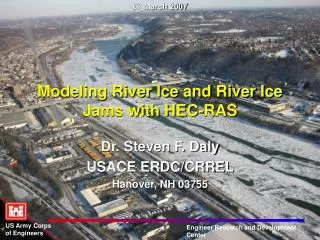
07 March 2007. Modeling River Ice and River Ice Jams with HEC-RAS. Dr. Steven F. Daly USACE ERDC/CRREL Hanover, NH 03755. Overview of Lecture. River Ice Hydraulics Modifications to Manning’s equation Available flow area Composite roughness Hydraulic radius

E N D
07 March 2007 Modeling River Ice and River Ice Jams with HEC-RAS Dr. Steven F. Daly USACE ERDC/CRREL Hanover, NH 03755
Overview of Lecture • River Ice Hydraulics • Modifications to Manning’s equation • Available flow area • Composite roughness • Hydraulic radius • standard step backwater procedure with ice • Entering Ice Data in HEC-RAS • Wide river ice jams – Theory • Simulating Ice jam with RAS
Manning’s Equation Manning equation for steady flow, expressed for the flow velocity or the total discharge, Q
d B Manning’s Equation with Ice River ice covers always float at hydrostatic equilibrium. Or more exactly Non-hydrostatic pressure will always be temporary and relatively short lived and for practical applications can be ignored.
d B Manning’s Equation with Ice: Area and Hydraulic Radius Adjust the terms of the Manning’s equation to account for the presence of ice Recall that for open water R ~ d
Ice region Bed region Max velocity Velocity Profile under steady flow conditions If we assume that the average flow velocity in the ice region and the bed region are equal; And we assume Manning’s equation applies to each; And we assume the energy grade line is the same in both; Composite Roughness value ni nb Sabaneev Formula
Suggested Range of Manning’s n Values for Ice Covered RiversThe suggested range of Manning’s n values for a single layer of ice Type of Ice Condition Manning’s n value Sheet ice Smooth 0.008 to 0.012 Rippled ice 0.01 to 0.03 Fragmented single layer 0.015 to 0.025 Frazil ice New 1 to 3 ft thick 0.01 to 0.03 3 to 5 ft thick 0.03 to 0.06 Aged 0.01 to 0.02
Thickness Manning’s n value ft Loose frazil Frozen frazil Sheet ice 0.3 - - 0.015 1.0 0.01 0.013 0.04 1.7 0.01 0.02 0.05 2.3 0.02 0.03 0.06 3.3 0.03 0.04 0.08 5.0 0.03 0.06 0.09 6.5 0.04 0.07 0.09 10.0 0.05 0.08 0.10 16.5 0.06 0.09 The suggested range of Manning’s n values for ice jams
Manning’s Equation with Ice for Rectangular Channels At least 32% increase in total depth due to ice cover at uniform flow
Standard Step Backwater Method d2 d1 Z2 Z1
Energy Losses with Ice The energy head loss can be expressed as the product of the mean friction slope, , and the distance between cross sections, L The friction slope is found from Manning’s equation. Often it is Re-written in the following form, using the conveyance, K
Energy Losses with Ice K can be expanded as There are several means of estimating the mean friction slope. The Simplest is probably the mean of the upstream and downstream slope Or other combination method
Entering ice data • All ice data is entered using the geometry data window. • The most basic way to enter the ice data is cross section by cross section using the cross section editor
Pull down menus Cross section editor Short cut Buttons River schematic
Enter the ice cover thickness Enter the Manning’s n values Ice jam data will be covered in the next section
Ice cover data • Using this window the ice cover properties can be entered for each cross section • However this has been found to be a long and tedious process • So a short cut table has been developed • Return to the main geometry editor
Ice cover table • This table allows a fast way to enter the ice cover thickness and roughness at all the cross sections at once. • As long as the “ice jam channel” is set to “no” or (n) for all cross sections the program will calculate the flow properties using the ice properties that are entered.
Ice thickness in LOB, channel and ROB Manning’s n value in LOB, channel and ROB As long as all sections are “n” the ice cover properties entered will be used.
Ice data • Once the ice data has been entered the geometry file can be resaved with a new name to separate the open water from the ice covered geometry data. This can be done by selecting Save Geometry Data AS from the “Geometric Data” windowunder the “file” menu
Shear Resistance at Banks Internal Shear Strength (Plan View) Wind stress Shear From Water Flow (Profile) Downstream Component of Jam Weight Forces on an Ice Jam
Transition Uniform Equilibrium Section Transition Uniform Solid Ice Cover Maximum depth given by equilibrium section Ice Jam Sections
Ice Jam Force Balance For Wide River Jam Longitudinal Force Gravity component, Sw = water surface slope Fluid shear stress Bank Shear Stress
Vertical StressGranular ice mass floating at hydrostatic equilibrium z Average vertical stress Longitudinal stress Transverse stress Bank shear
Estimating the ice jam thickness based on the complete ice jam force balance equation Starting with the ice jam force balance equation:
Modeling ice jams • HEC-RAS simulates river ice jams by adjusting the jam thickness until the ice jam force balance equation and the standard step backwater equation are satisfied.
Ice Jam Force Balance Solution Procedure • Ice Jam Force Balance is solved from upstream to downstream • Assume an jam thickness at the next downstream section • Iterate until a solution is found. (25 Iterations max.) Relaxation procedure used. • Ice cannot completely block cross section at assure this a maximum flow velocity allowed under ice (5 fps default) • Minimum ice jam thickness based on the thickness set by the user
Global Solution Procedure • Initial Backwater calculations downstream to upstream using entered ice thickness • Ice Jam Force Balance solved upstream to downstream using flow values determined from backwater analysis • Backwater and Ice Jam Force Balance are alternated until a solution is achieved • The ice jam thickness is allowed to change only 25% of calculated required change in each iteration. (Global relaxation)
Global Solution Convergence • Water surface elevation at any cross section changes less than 0.06 ft, or a user supplied tolerance, and the ice jam thickness at any section changes less than 0.1 ft, or a user supplied tolerance, between successive solutions of the ice jam force balance equation. • A total of 50 iterations (or a user defined maximum number) are allowed for convergence.
Modeling Wide River Ice Jam • User specifies (globally or at each section) • Extent of the jam • Limit jam to channel or include overbanks • Material properties of the jam • Internal friction angle (45º) • Jam Porosity (0.4) • K1 (.33) • Maximum flow value under the jam (5 fps) • Manning’s n or let RAS estimate
Selecting the ice jam location • The user must select where an ice jam will be located. HEC-RAS cannot determine on its own where a jam will be. • The ice cover editor available from the cross section data window, or the ice cover table, available from the geometry data window can be used to locate the jam.
Selecting the ice jam location • The user must also determine if the jam will be confined to the channel or be allowed to extend into the over banks.
Selecting the ice jam location Confining the jam to the channel is appropriate where • the water levels do not reach the overbank • The river ice is confined to the channel by trees • The overbank areas are very broad and an ice jam could not form in these areas
Ice jam confined to channel Confined to Channel LOB ROB
Selecting the ice jam location • If the jam is allowed to enter the overbank area, then the flow properties of the overbank and the channel are combined to determine the average flow properties acting on the jam.
Select ice jam option by setting where the ice jam will be located By selecting Channel or Over banks These boxes will become available Channel plus over banks Channel
The ice jam option can also be set in the ice cover table. This is done by changing the no’s, n, to yes’s, y, in the appropriate column. The user must select if the ice jam is confined to the channel or will include both the channel and the over banks. Change each cross section individually. The values cannot be set to y or n all at once, as the numeric values can. Channel Channel plus over banks
Selecting ice jam location • Remember: there must be section with fixed ice thickness at the upstream and downstream end of the jam. • Therefore, every cross section can not be set to yes. There must be at least one section with no at the upstream and downstream ends of the jam.
Ice Jam Parameters • = angle of internal friction • ’ = density of ice • e = porosity of jam • k1 = ratio of lateral to longitudinal pressure
’ = density of ice = angle of internal friction e = porosity of jam k1 = ratio of lateral to longitudinal pressure The user can enter the values on the ice cover editor for each cross section individually. Note that default values of the parameters have already been entered.
Ice jam parameters • The user can also set the ice jam parameters globally using the ice cover table. Note that default values of the parameters have already been entered.
The numeric values can be set globally, like the ice thickness and roughness values k1 = ratio of lateral to longitudinal pressure e = porosity of jam = angle of internal friction ’ = density of ice
Manning’s roughness of jam • The user can either fix the Manning’s n value for the jam or let HEC-RAS estimate the value based on Nezhikovsky’s formula
Estimation of Manning’s n for Ice Jamusing Nezhikovsky’s formula t >1.5 ft t <1.5 ft
If the box below is checked, these values are considered fixed, and will be used By un-checking this box, the user allows RAS to estimate the Jam roughness