Download

1 / 19
200 likes | 354 Vues
RiskCity Introduction to Frequency Analysis of hazardous events. Extreme Events. “Man can believe the impossible. But man can never believe the improbable.” - Oscar Wilde.

E N D
RiskCityIntroduction to Frequency Analysis of hazardous events ISL 2004
Extreme Events “Man can believe the impossible. But man can never believe the improbable.” - Oscar Wilde “It seems that the rivers know the [extreme value] theory. It only remains to convince the engineers of the validity of this analysis.” –E. J. Gumbel Linda O. Mearns NCAR/ICTP
Objective of FA exercise • The objective of this exercise is to practice different methods of frequency analysis for floods and for earthquakes and to gain insight in magnitude – frequency relationship. • Keep in mind that the methods presented in this exercise are just a selection of all existing methods. • In this exercise ILWIS is not being used. ISL 2004
M-F relationship • Magnitude-frequency relationship is a relationship where events with a smaller magnitude happen more often than events with large magnitudes. • Magnitude is related to the amount of energy released during the hazardous event, or refers to the size of the hazard. • Frequency is the (temporal) probability that a hazardous event with a given magnitude occurs in a certain area in a given period of time. ISL 2004
M-F relationship • The M – F relationship does hold true for many different disaster types, but as can be seen in the table, not for all: ISL 2004
Flooding • Return period/exceeding probability • Extreme value distribution by Gumbel method • Intensity-duration-frequency relationships
3 1 1 5 Between 1935 and 1978: 9 events 6 8 Intervals, ranging from 1 to 16 years 16 5 4 Flooding Return period/exceeding probability Maximum daily preciptation (mm) What is the return period of a rain event over a 100 mm/day ? The sum of the intervals = 4 + 1 + 1 + 16 +3 + 6 + 5 + 5 = 41 Average = 41/8 = 5.1 years Annual exceedence probability of a rain event over 100 mm/day = 100 / 5.1 = 19.5 %
Flooding Return period/exceeding probability For the average annual risk! Q100 has a greater probability of occurring during the next 100 yrs (63%) than during the next 5 years ( 5%)
Flooding Frequency Analysis
12 10 8 Frequency 6 4 2 0 800 450 500 550 600 750 850 900 950 650 700 Rainfall classes (mm) Flooding Frequency Analysis
X Flooding Frequency Analysis P(R < 642) = 0.5 Mean: 642 mm Standard deviation: 110 mm P(R > 642) = 0.5 P(532 < R < 752) = 0.683 P(422 < R < 862) = 0.954 P(312 < R < 972) = 0.997 0.683 0.954 0.997 -2 +2 -3 -1 +1 +3
Flooding Unfortunately, a large amount of events is right skewed; • Magnitude of events are absolutely limited at the lower end and not at the upper end. The infrequent events of high magnitude cause the characteristic right-skew • The closer the mean to the absolute lower limit, the more skewed the distribution become • The longer the period of record, the greater the probability of infrequent events of high magnitude, the greater the skewness
12 10 8 Frequency 6 4 2 0 800 450 500 550 600 750 850 900 950 650 700 Rainfall classes (mm) Flooding • The shorter the time interval of recording, the greater the probability of recording infrequent events of high magnitude, the greater the skewness • Other physical principles tend to produce skewed frequency distributions: e.g. drainage basin size versus size of high intensity thunderstorms.
Flooding Solution to right-skewness: Use Extreme Value transform (other names: Double exponential transform or Gumbel transformation): • Rank the values from the smallest to the largest value • Calculate the cumulative probabilities: P=R/(N+1)*100% • Plot the values against the cumulative probability on probability paper and draw a straight line (best fit) through the points • From the line, estimate the standard deviation and mean • Estimate all other required probabilities versus values
Flooding Extreme value distribution by Gumbel method
Flooding Intensity-duration-frequency relationships Intensity Duration IDF curves are calculated for a certain station and it cannot be extrapolated to other areas.
Earthquakes Per day 0.5 4 36 360 (every 4 minutes….) 3600 (every 24 seconds….)
The Gutenberg-Richter Relation Earthquakes log N(M) = a – bM Gutenberg-Richter plots are made for various data sets all over the world, and most of them end up having a b value very close to 1, usually slightly less.