Download
1 / 23
450 likes | 1.3k Vues
CUMULATIVE FREQUENCY AND OGIVES. AS 10.4.1 (a) Collect, organise and interpret univariate numerical data in order to determine measures of dispersion, including quartiles, percentiles and the interquartile range AS 11.4.1 (a) Calculate and represent measures of

E N D
AS 10.4.1 (a) Collect, organise and interpret univariate numerical data in order to determine measures of dispersion, including quartiles, percentiles and the interquartile range AS 11.4.1 (a) Calculate and represent measures of central tendency and dispersion in univariate numerical data by drawing Ogives
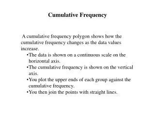
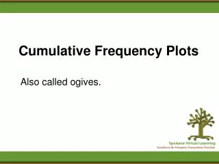
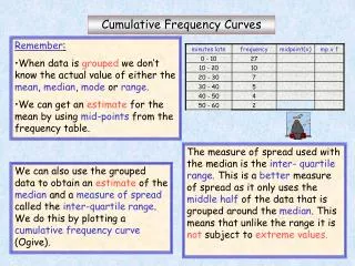
Ogives • The word ogive is used to describe various smooth curved surfaces. • S-shaped. • Cumulative frequency curve.
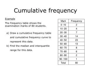
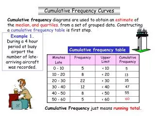
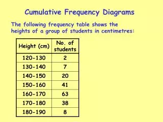
Cumulative Frequency Table • In a frequency table you keep count of the number of times a data item occurs by keeping a tally. The number of times the item occurs is called the frequency of that item. • In a frequency table you can also find a ‘running total’ of frequencies. This is called the cumulative frequency. It is useful to know the running total of the frequencies as this tells you the total number of data items at different stages in the data set.
Check that the final total in the cumulative column is the same as the total number of students
Activity 1 • b) 34 learners c) 82 – 34 = 48 learners d) 77 learners • a) b) i) 23 learners ii) 3 learners iii) 25 learners
A cumulative frequency table can be drawn up from: • Ungrouped data (see page 3) • Grouped discrete data (see page 4) • Grouped continuous data (see page 5)
Activity 2 – question 1 • 28 • 59 • 21 + 10 = 31 or 90 – 59 = 31
Activity 2 – question 2 • The way the interval is given 0<x ≤ 10 versus 1 – 10 • 15 learners • 16 + 11 = 27, or 140 – 113 = 27 • Couldn’t
We represent data given on a frequency table by drawing • A broken line graph • A pie chart • A bar graph • A histogram • A frequency polygon We represent data given on a cumulative frequency table by drawing a cumulative frequency graph or ogive
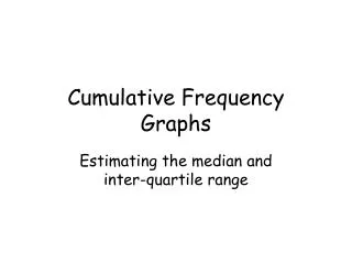
Drawing a Cumulative Frequency Curve or Ogive • Running total of frequencies • S – shape • Starts where frequency is 0.
Activity 4 – question 1 • 59 learners • Yes • 90 – 59 = 31 learners
THE MEDIAN AND QUARTILES FROM A CUMULATIVE FREQUENCY TABLE Suppose we have the marks of 82 learners. We can divide the marks into four groups containing the same number of marks in the following way:
These values can be found in the cumulative frequency table by counting the data items: The 21st student is here. Q1= 5 The 41st and 42nd students are here. Median = 7 The 62nd student is here. Q3= 8
The Median and Quartiles from an Ogive Q3 is the 62nd value Estimate of upper quartile is read here. Q3≈8 Median is the 41½th value Estimate of median is read here. M ≈ 7 Q1 is the 21st value Estimate of lower quartile is read here. Q1≈ 5
Percentiles • Deciles:They divide the data set into 10 equal parts • Percentiles : They divide the data set into 100 equal parts • The median is the 50th percentile. This means 50% of the data items are below the median • Q1 = 25th percentile. This means 25% of the data items are below Q1 • Q3 = 75th percentile. This means 75% of the data items are below Q3
Percentiles should only be used with large sets of data. Example: The 16th percentile of the data on the previous page is found like this: 16% of 82 = 13,12 On vertical axis find 13 then read across to curve and then down to horizontal axis 16th percentile 4 This means 16% of the class scored 4 marks or less.
Activity 5 • (a) 10% of 82 = 8,2 10th percentile ≈ 3 90% of 82 = 73,8 90th percentile ≈ 9 (b) 80% of the marks lie between 3 and 9. (c) 50% of the class got 7 or less out of 10 for the test. 2. (a) 50th (b) 25th (c) 75th
Activity 5 – question 3 continued • Median is the 50½ th term. It lies in the interval 41 – 50. Median ≈ 45,5 • Lower quartile is the 25½ th term. It lies in the interval 31 – 40. Q1 ≈ 35,5 Upper quartile is the 75½ th term. It lies in the interval 51 – 60. Q3 ≈ 55,5