Download
1 / 71
710 likes | 928 Vues
Innovation Approach to the Identification of Causal Models in Time Series Analysis. T. Ozaki Institute of Statistical Mathematics. ( Wold, Kolmogorov, Wiener, Kalman, Kailath). Innovation Approach. ( Box-Jenkins , Akaike etc.). Causal Model. Ozaki(1985, 1992, 1995, 2000).

E N D
Innovation Approach to the Identification of Causal ModelsinTime Series Analysis T. Ozaki Institute of Statistical Mathematics
(Wold, Kolmogorov, Wiener, Kalman, Kailath) Innovation Approach (Box-Jenkins , Akaike etc.) Causal Model Ozaki(1985, 1992, 1995, 2000)
What causes the time-dependencyingeophysical time series? Geophysical Dynamical System
Three topics in time series 1. Nonlinear time series Dynamical Systems 2. Non-Gaussian time series Dynamical Systems & Shot Noise 3. Spatial time series Spatial Dynamics Innovation Approach
Ozaki&Oda(1976) Dynamical System & Time Series Model Restoring force ∝ W・GM sin x W・GM sin x x : for small x W・GM sin x x - 1/6 x3 : for large x xt D.S. nt
ExpAR Model • Smaller prediction errors than AR models. 2. Mechanical interpretation Ozaki&Oda(1976)
Natural frequency n(t) x(t) nt xt f0
Idea : Dynamic eigen-values 1. Duffing equation 2. van der Pol equation
Make it non-explosive ! Explosive ! Non-explosive ! Make it stay inside for large xt-1 !
Ozaki(1985) ExpAR Singular points
Ozaki(1985) ExpAR-Chaos
ExpAR Models & non-Gaussian distributions Ozaki(1985) : Stable singular points : Unstable singular points
Distribution of ExpAR process nt+1 ExpAR xt+1 non-Gaussian Gaussian white noise
Time discretizationsofdx=f(x)dt+dw(t) Euler scheme Heun scheme Runge-Kutta scheme Explosive nonlinear AR model ! Any non-explosive scheme ?
i). Ozaki(1984) L.L. scheme ii). Ozaki(1985) iii). Biscay et al.(1996) iv). Shoji & Ozaki(1997) Characteristics 1. Simple 2. A-stable
(Wold, Kolmogorov, Wiener, Kalman, Kailath) Innovation Approach (Box-Jenkins , Akaike etc.) Causal Model Ozaki(1985, 1992, 1995, 2000)
Data Three types of models Time Series Models (ExpAR, neural net etc.) Dynamic Phenomena Stochastic Dynamical Systems Dynamical Systems
Applications 1. Non-Gaussian time series and nonlinear dynamics 2. Estimation of dx=f(x)dt+dw(t) dx/dt=f(x) 3. RBF-Neural Net vs ExpAR, RBF-AR modeling 4. Spatial time series modeling
Application-(1)Non-Gaussian time seriesandnonlinear dynamics Does non-Gaussian-distributed time series mean non-Gaussian prediction errors? Not Necessarily !
Distribution of ExpAR process nt+1 ExpAR xt+1 non-Gaussian Gaussian white noise
Ozaki(1985,1990) Same DistributionDifferent Dynamics a=3,b=1 i) a=3,b=1 ii) a=3,b=1 iii)
(Ozaki, 1985,1992) Gamma-distributed Process(Type II) Mechanism • x(t) is generated from i) Gaussian white noise ii) Nonlinear Dynamics iii)Variable Transformation
This implies the validity of innovation approach Non-Gaussian time series Gaussian white noise
When residuals of your model arenon-Gaussianlooking,what would you do? 1.Introducenon-Gaussian noisemodel Bayesian Approach 2.Improve theCausal Model so that it produces Gaussian residuals Innovation Approach
Application-(3)RBF-AR & RBF Neural Net ExpAR model is not suffucient More complicated dynamics, i.e. fk(x(t-1)) RBF-AR y-dependent system characteristics, i.e. fk(x(t-1), y(t-1)) RBF-ARX
RBF-AR & RBF Neural Net More complicated fk(x(t-1)) f(xt ) RBF-AR(p,d,m) 1 xt Z1 0 Z2 RBF- Neural Net (p,d,m)
Application - (2) Estimation of Numerical examples 1. Rikitake chaos, ( Geophysics) 2. Zetterberg Model (Brain Science) 3. Dynamic Market model ( Finance)
How to identify ? from
Frost & Kailath(1971)’s theorem : Gaussian white noise Non-Gaussian time series Nonlinear Filter Gaussian white noise
Likelihood Calculation Innovation Approach : Gaussian white noise Frost & Kailath(1971) How to obtain nt and snt2 ? Nonlinear Filter
Relations to Jazwinski(1970)’s scheme Innovation Approach Calculate p(xk|zk) & p(zk|zk-1) etc. by Local Gauss model. L.L.
Two Choices for Approximation 1) Local Gauss 2) Local non-Gauss Use of Fokker-Planck equation. Computationally 1) is super more efficient than 2)
Advantages of the L.L. Scheme See B.L.S.Prakasa Rao(1999) Statistical Inference for Diffusion Type Processes H.Schurz(1999) A Brief Introduction To Numerical Analysis of (Ordinary) Stochastic Differential Equations Without Tears Essence is Stability & Efficiency
Numerical examples 1. Rikitake chaos ( Geophysics) 2. Zetterberg Model (Brain Science) 3. Dynamic Market model ( Finance)
Identification of the chaotic Rikitake model(Ozaki et at. 2000) Simulation obtained by the LL scheme Rikitake(1957), Ito(1982)
Identification Results Simulated and estimated states
Three types of parameters Structured-parameter optimization for M.L.E. method 1. Peng & Ozaki(2001) 2. 3.
Initial values & Estimated States : optimized : optimized : not optimized : optimized
Initial values & Innovations : optimized : optimized : not optimized : optimized
Reality in Data Analysis 1.Zero prediction errors are not possible to attain even with nonlinear causal (chaos) models. • Time - inhomogeneous residuals • Gaussian white residuals + a few outliers 2.Residuals of ARIMA models are usually almost Gaussian, but not always. • Generally distributed residuals are rare ! (We don’t see bi-modally distributed residuals)
Whitening filter-1 Whitening filter-2 Obvious Choice A question is whether it is possible to find a perfect deterministic model for the data x1,x2,…,xN Causal Model-1 Causal Model-2 (Stochastic Model) (Deterministic Model)
Application - (4) Spatial time series modeling
Example : Data assimilationin meteorology States on the lattice points (i,j) Estimation Observations
Rabier et al(1993) Mutual understanding : on the way Variationalmethod (4D-Var ) Ide & Ghil(1997) Closed system Perfect model with Observation errors Penalized Least Squares method • Open system • Model errors as well as Observation errors
Similar principles Variational method (4D-Var ) Closed system Perfect model with observation errors Penalized Least Squares method Open system Model errors as well as observation errors Sequential method (Extended Kalman Filter MLE ) Open system Model errors as well as observation errors (similar to P.L.S. but not the same!)
Hidden approximations behind perfect-model assumptions Infinite dimensional state Finite dimension ( Model error) Open universe Closed system ( Model error) Nonlinear dynamics Numerical Approximation ( Model error)