Download
1 / 39
440 likes | 743 Vues
Topographic correction of Landsat ETM-images. Markus Törmä Finnish Environment Institute Helsinki University of Technology. Background. CORINE2000 classification of whole Finland Forested and natural areas are interpreted using Landsat ETM-image mosaics. Background.

E N D
Topographic correction of Landsat ETM-images Markus Törmä Finnish Environment Institute Helsinki University of Technology
Background • CORINE2000 classification of whole Finland • Forested and natural areas are interpreted using Landsat ETM-image mosaics
Background • Estimation of continuous variables like tree height and crown cover • Continuous variables are transformed to discrete CORINE-classes using IF-THEN-rules • According to the test classificatios, there is need for a SIMPLE topographic correction method in Lapland
Background • Landsat ETM 743, Kevo and digital elevation model
Background Tested methods: • Lambertian cosine correction • Minnaert correction • Ekstrand correction • Statistical Empirical correction • C-correction Tests: • Maximum Likelihood-classification to land cover classes • Comparison of class statistics between and within classes • Linear regression to estimate tree height, tree crown cover and vegetation cover • Estimation of tree crown cover and height using Proba-software (VTT)
Topografic correction • Imaging geometry changes locally causing unwanted brightness changes • E.g. deciduous forest looks like more bright on the sunny side that the shadow side of the hill • Reflectance is largest when the slope is perpendicular to the incoming radiation
Topografic correction • Intensities of image pixels are corrected according to the elevation variations, other properties of the surface are not taken into account • The angle between the surface normal and incoming radiation is needed ”Illumination image”
Example • Landsat ETM (RGB: 743) and digital elevation model made by National Land Survey
Example • Landsat ETM (RGB: 743) and Illumination image
Example • Correlation between pixel digital numbers vs. illumination varies between different channels
Lambert cosine correction • It is supposed that the ground surface is lambertian, i.e. reflects radiation equal amounts to different directions LC = LO COS(sz) / COS(i) • LO: original digital number or reflectance of pixel • LC: corrected digital number • sz: sun zenith angle • i: angle between sun and local surface normal
Lambert cosine correction • Original and corrected ETM-image • Note overcorrection on the shadow side of hills
Minnaert correction • Constant ksimulates the non-lambertian behaviour of the target surface LC = LO [ COS(sz) / COS(i) ]k • Constant k is channel dependent and determined for each image
Minnaert correction • Original and corrected ETM-image • Still some overcorrection
Ekstrand correction • Minnaert constant k varies according to illumination LC = LO [ COS(sz) / COS(i) ]k COS(i)
Ekstrand correction • Original and corrected ETM-image
Determination of Minnaert constant k • Linearization of Ekstrand correction equation: -ln LO = k cos i [ ln (cos(sz) / cos(i)) ] – ln LC • Linear regression • Line y = kx + b was adjusted to the digital numbers of the satellite image y = -ln LO x = cos i [ln(cos(sz) / cos(i))] b = -ln LC
Minnaert constant k • Samples were taken from image • Flat areas were removed from samples • In order to study the effect of vegetation to the constant, samples were also stratified into classes according to the NDVI-value
Minnaert constant k • NDVI classes and their number of samples
Minnaert constant k • Correlation between pixel digital numbers vs. illumination varies between different NDVI-classes on the channel 5
Determination of Minnaert constant k • Determined constants k and corresponding correlation coefficients r for different channels
Statistical-Empirical correction • Statistical-empirical correction is statistical approach to model the relationship between original band and the illumination. LC = LO– m cos(i) m: slope of regression line • Geometrically the correction rotates the regression line to the horizontal to remove the illumination dependence.
Statistical-Empirical correction • Original and corrected ETM-image
C-correction • C-correction is modification of the cosine correction by a factor C which should model the diffuse sky radiation. LC = LO [ ( cos(sz) + C ) / ( cos(i) + C ) ] • C = b/m • b and m are the regression coefficients of statistical-empirical correction method
C-correction • Original and corrected image
Determination of slope m and intercept b • Regression coefficients for Statistical-empirical and C-correction were determined using linear regression • Slope of regression line m and intercept b were determined using illumination (cos(i)) as predictor variable and channel digital numbers as response variable
Determination of slope m and intercept b • Slopes m and correlation coefficients r for different channels
Maximum Likelihood-classification • Ground truth: Lapland biotopemap
Maximum Likelihood-classification • Accuracy measures: overall accuracy (OA), users’s and producer’s accuracies of classes for training (tr) and test (te) sets • Original image: Oatr 57.2%, Oate 48.2% • Cosine correction: Oatr 60.9%, Oate 51.9%
Maximum Likelihood-classification • In the case of test set, the correction methods usually increased classification accuracy compared to original image • Stratification using the NDVI-class increases classification accuracy of test pixels in the cases of Ekstrand and Statistical-Empirical correction.
Comparison of class statistics • Jefferies-Matusita decision theoretic distance: distance between two groups of pixels defined by their mean vectors and covariancematrices • Distances were compared between classes and within individual classes
Comparison of class statistics Between-class-comparison • 14 Biotopemapping classes • separability should be as high as possible Within-class-comparison • 7 Biotopemapping classes • classes were divided into subclasses according to the direction of the main slope • separability should be as low as possible
Comparison of class statistics Between-class-comparison • Cosine correction and original image best Within-class-comparison • Statistical-Empirical correction best, Cosine correction and original image worst • The effect of correction is largest for mineral soil classes and smallest for peat covered soils. • Stratification using the NDVI-class decreases the separability of subclasses
Linear regression • Estimate tree height, tree crown cover and vegetation cover Ground survey • 300 plots in Kevo region, Northern Lapland • Information about vegetation and tree crown cover, tree height and species
Linear regression Tree height • Statistical-Empirical best • Stratification decreases the correlation a little Tree crown cover • Cosine and C-correction best • Stratification decreases the correlation a little Vegetation cover • C- and Minnaert correction best
Estimation of tree crown cover and height • Proba-software (Finnish National Research Center) • Training (3386) and test (1657) compartments from Lapland Biotopemap, compartmentwise averages • Tree height and crown cover were estimated for image pixels and compartment averages computed • Error measures: Bias, Root Mean Squared Error, Correlation Coefficient
Estimation of tree crown cover and height Tree height • C-correction best • Topographic correction and stratification decreases estimation error Tree crown cover • Ekstrand correction best • Topographic correction and stratification decreases estimation error
Conclusion • Topographic correction improves classification or estimation results • But methods perform differently and their performence depends on task at hand • In some cases correction even make results worse so it is difficult to choose the best method
Conclusion • The best correction methods seem to be C-correction and Ekstrand correction • The stratification according to the NDVI-class improves results in some cases, depending on the used experiment