Time series ( TS )
Time series ( TS ). What is the time serie ??. data about the socio - economic phenomenon - in chronological order in time properly assembled time series data must meet the comparability of data: in time (the same length of periods) in space (the same territorial units, regions)

Time series ( TS )
E N D
Presentation Transcript
Time series (TS) doc.Ing. Zlata Sojková, CSc.
What is the time serie?? data about the socio - economic phenomenon - in chronological order in time properly assembled time series data mustmeet the comparability of data: • in time (the same length of periods) • in space (the same territorial units, regions) • and substantive comparability (same methodology) doc.Ing. Zlata Sojková, CSc.
Denote the value of the investigated variable: y1, y2 , y3 , ... yt …… yT, wheret = 1, 2, …. T,T is the number of periods, t is formal time variable, which specifies the order of the value , e.g. GDP SR per capita. Years 95-99 v US$ doc.Ing. Zlata Sojková, CSc.
Basic types of time seriesdepending on the nature of data doc.Ing. Zlata Sojková, CSc.
By the length of the period we distinguish: • Long-term time series- yearly data, etc. • Short-term time series- quarterly, monthly data....etc... doc.Ing. Zlata Sojková, CSc.
Basic characteristics of time series analysis • Absolute rate of growth (decline): • absolute increase (decline) – first differences y t = y t - y t -1 • second first differences (acceleration) y t 2 = y t - y t -1 doc.Ing. Zlata Sojková, CSc.
Relative rate of growth • coefficients of growth: k t = y t / y t - 1 • coefficient of increase: k t = k t - 1 • growth rate (growth coef .in % ): Tt = k t . 100 • Increase rate: Tt =Tt - 100, resp. Tt = (k t - 1 ) . 100 doc.Ing. Zlata Sojková, CSc.
GDP SR for years rr.95-99 in US$ per capita and year. In 1997 compared to 96 increasedGDP per capita on 108,12% In 1997 compared to 96 increased GDP per capita by 8,12% doc.Ing. Zlata Sojková, CSc.
From individual growth rates can be calculated: average growth rate _ 4 k = (1,148.1,081. 1,003 . 0,974)= 1.0493 For the period 95-99 was growth of GDP in SR per year approximately 4,9% doc.Ing. Zlata Sojková, CSc.
Components of time series Time series are created as the effect of important and not important factors on investigated phenomenon. These factors can be divided: • Trend– determine the main direction of development t.j. trend in TS (Tt ) • Periodic – cause regular fluctuations around the trend values of TS, can be divided: • Cyclic(C t )- in long-term TS (economic cycles) • Seasonal (S t )-in short-term TS (seasonal fluctuations of prices, seasonal demand…..), doc.Ing. Zlata Sojková, CSc.
Random effects(E t ) – random, iregular. These factors affect the development of each investigated variable in statistics. => We can decompose TS into three components: • Trend (Tt ) • Periodic(C t ), resp. (S t ) • Random (E t ) Between components may be: • Adittive relationship: Yt = T t + St + Et • Multiplicative relationship: Yt = T t . St . Et doc.Ing. Zlata Sojková, CSc.
Analysis of trend andseasonal component (if occurs in TS) Using standard decomposition approach Analysis of trend in TS Analysis of trend using decomposition approach is based on: • analytical smoothing of investigated values by appropriate trend function. • analogy to the simple regression analysis, the estimated values are a function of time variable t, yt , = f (t) • „trend function“ is then used not only to evaluating the quality of forecasts "ex post", but also to forecast ex-ante doc.Ing. Zlata Sojková, CSc.
Historical data „Ex ante“ prognosis doc.Ing. Zlata Sojková, CSc.
Statistical evaluation of appropriatness of function • using index of correlation i yt, resp. • index of determinationiyt2 • Which reflects the quality of “ex-post” forecast • Priority is assesment of the fittnes of trend function. It is necessaryto consider future development of examined variable y. doc.Ing. Zlata Sojková, CSc.
Analysis of seasonal component in TS Decomposition approach It is assumed: • Multiplicative model of TS: Yt = Tt . St . Et • Analysis of trend in TS (if present) by suitable trend function: Tt = yt, = f(t) • Analysis of seasonal component using seasonal indices: where y t , are values obtained from fitted trend function for t = 1,2…T doc.Ing. Zlata Sojková, CSc.
In table are data about Revenue of chosen company for 3 years. Analyse development of revenues in recent years and make forecast for year 1990. Yt = Tt . St . Et Tt = yt, = f(t) We create variable t = 1,2,…,12 How to make Forecast for 1999 ? doc.Ing. Zlata Sojková, CSc.
Development of revenues (obvious seasonal fluctuations) doc.Ing. Zlata Sojková, CSc.
Procedure for analysis and prediction: • First, we analyze the trendusing suitable trend function. From the chart can be concluded that linear function is sufficient. • We will use Excel (Tools- data Analysis -Regression) • We calculate „predicted“ values according to trend function (also for year 1990) • Seasonal Indices St are calculated by dividing real value of revenuesy tby value y t ‘ predicted according to trend function • We make average of seasonal indices(to objectify seasonal component) and correct them for the sum of 4 (correction for accurancy) doc.Ing. Zlata Sojková, CSc.
Result of trend analysis Aproximately 60% of revenue variability is explained by trend, rest 40% is the variability caused by seasonal and random fluctuations We use trend function coefficients for „ex-post“ and „ex-ante“ forecast of trend doc.Ing. Zlata Sojková, CSc.
Analysis of seasonality and forecast Forecast Y t ‘ . Stpriem. Seasonal indices Predicted values of trend Forecast for trend and seasonality Forecast Of trend doc.Ing. Zlata Sojková, CSc.
Real values „ex-ante“ forecast for trend and seasonality Forecast of trend doc.Ing. Zlata Sojková, CSc.
It was just briefly introduction in TS analysis….. … …good luck... doc.Ing. Zlata Sojková, CSc.

