Download
1 / 48
480 likes | 596 Vues
DNA, RNA and protein are an alien language ... We try to cryptographically attack this language ... we want to decipher both its meaning and its history …. Fortunate the genetic code is alphabetic … susceptible to perform string comparisons and pattern recognition.

E N D
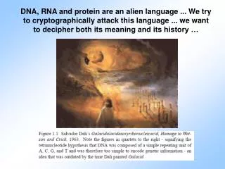
DNA, RNA and protein are an alien language ... We try to cryptographically attack this language ... we want to decipher both its meaning and its history …
Fortunate the genetic code is alphabetic … susceptible to perform string comparisons and pattern recognition We do not have to understand the languaje to identify patterns: “klaatu barada nikto”
Pairwise Sequence Alignment • Principles of pairwise sequence comparison • global / local alignments • scoring systems • gap penalties • Methods of pairwise sequence alignment • window-based methods • dynamic programming approaches
Pairwise Sequence Alignment: How to? A T T C A C A T A T A C A T T A C G T A C Sequence 2 Sequence 1
Dotplot: A dotplot gives an overview of all possible alignments A T T C A C A T A T A C A T T A C G T A C Sequence 2 Sequence 1
Dotplot: In a dotplot each diagonal corresponds to a possible (ungapped) alignment A T T C A C A T A T A C A T T A C G T A C Sequence 2 Sequence 1 T A C A T T A C G T A C A T A C A C T T A One possible alignment:
Pairwise Sequence Alignment • Principles of pairwise sequence comparison • global / local alignments • scoring systems • gap penalties • Methods of pairwise sequence alignment • window-based methods • dynamic programming approaches
Window-based Approaches • Word Size • Window / Stringency
Word Size Algorithm T A C G G T A T G A C A G T A T C Word Size = 3 C T A T G A C A T A C G G T A T G T A C G G T A T G A C A G T A T C T A C G G T A T G A C A G T A T C T A C G G T A T G A C A G T A T C
Window / Stringency Window = 5 / Stringency = 4 T A C G G T A T G T C A G T A T C C T A T G A CA T A C G G T A T G T A C G G T A T G T C A G T A T C T A C G G T A T G T C A G T A T C T A C G G T A T G T C A G T A T C
Considerations • The window/stringency method is more sensitive than the wordsize • method (ambiguities are permitted). • The smaller the window, the larger the weight of statistical • (unspecific) matches. • With large windows the sensitivity for short sequences is reduced. • Insertions/deletions are not treated explicitly.
Insertions / Deletions in a Dotplot T A C T G T C A T T A C T G T T C A T Sequence 2 Sequence 1 T A C T G-T C A T | | | | | | | | | T A C T G T T C A T
Dotplot(Window = 130 / Stringency = 9) Hemoglobin-chain Output of the programs Compare and DotPlot Hemoglobin -chain
Dotplot(Window = 18 / Stringency = 10) Hemoglobin-chain Output of the programs Compare and DotPlot Hemoglobin -chain
Pairwise Sequence Alignment • Principles of pairwise sequence comparison • global / local alignments • scoring systems • gap penalties • Methods of pairwise sequence alignment • window-based approaches • dynamic programming approaches • Needleman and Wunsch • Smith and Waterman
Dynamic Programming Automatic procedure that finds the best alignment with an optimal score depending on the chosen parameters. Recursive solutions. We solve smaller problems first, and use those solutions to solve larger problems. Intermediate solutions are stored in a tabular matrix.
Basic principles of dynamic programming • - Initialization of alignment matrix: the scoring model • - Stepwise calculation of score values • (creation of an alignment path matrix) • - Backtracking (evaluation of the optimal path)
Initialization of Matrix(BLOSUM 50): A distance metric H E A G A W G H E E P -2 -1 -1 -2 -1 -4 -2 -2 -1 -1 A -2 -1 5 0 5 -3 0 -2 -1 -1 W -3 -3 -3 -3 -3 15 -3 -3 -3 -3 H10 0 -2 -2 -2 -3 -2 10 0 0 E 0 6 -1 -3 -1 -3 -3 0 66 A -2 -1 5 0 5 -3 0 -2 -1 -1 E 0 6 -1 -3 -1 -3 -3 0 66
Needleman and Wunsch(global alignment) Sequence 1: H E A G A W G H E E Sequence 2: P A W H E A E Scoring parameters: BLOSUM50 matrix Gap penalty: Linear gap penalty of 8
E E Creation of an alignment path matrix Idea:Build up an optimal alignment using previous solutions for optimal alignments of smaller subsequences • Construct matrix F indexed by i and j (one index for each sequence) • F(i,j) is the score of the best alignment between the initial segment x1...iof x up to xiand the initial segment y1...jof y up to yj • Build F(i,j) recursively beginning with F(0,0) = 0 H - E - A P G - G - H H E E - A A A W W Optimal global alignment:
Creation of an alignment path matrix H E A G A W G HEE 0 -8 -16 -24 -32 -40 -48 -56 -64 -72 -80 P -8 -2 -9 -17 -25 -33 -42 -49 -57 -65 -73 A -16 -10 -3 -4 -12 -20 -28 -36 -44 -52 -60 W -24 -18 -11 -6 -7 -15 -5 -13 -21 -29 -37 H -32 -14 -18 -13 -8 -9 -13 -7 -3 -11 -19 E -40 -22 -8 -16 -16 -9 -12 -15 -7 3 -5 A -48 -30 -16 -3 -11 -11 -12 -12 -15 -5 2 E -56 -38 -24 -11 -6 -12 -14 -15 -12 -9 1 HEAGAWGHE-E --P-AW-HEAE Optimal global alignment:
Creation of an alignment path matrix F(i, j) =F(i-1, j-1) + s(xi ,yj) F(i, j) = max F(i, j) = F(i-1, j) - d F(i, j) = F(i, j-1) - d F(i-1, j-1)F(i, j-1) F(i-1,j)F(i, j) HEAGAWGHE-E --P-AW-HEAE s(xi ,yj) -d -d
Creation of an alignment path matrix • If F(i-1,j-1), F(i-1,j) and F(i,j-1) are known we can calculate F(i,j) • Three possibilities: • xiand yj are aligned, F(i,j) = F(i-1,j-1) + s(xi ,yj) • xi is aligned to a gap, F(i,j) = F(i-1,j) - d • yjis aligned to a gap, F(i,j) = F(i,j-1) - d • The best score up to (i,j) will be the largest of the three options
Creation of an alignment path matrix H E A G A W G H E E 0 P A W H E A E -8 -16 -24 -32 -40 -48 -56 -64 -72 -80 -8 -16 -24 -32 -40 -48 -56 Boundary conditions F(i, 0) = -id F(j, 0) = -jd
F(i, j) = F(i-1, j-1) + s(xi ,yj) F(i, j) = max F(i, j) = F(i-1, j) - d F(i, j) = F(i, j-1) - d F(0,0) + s(xi ,yj) = 0 -2 = -2 F(1,1) = max F(0,1) - d = -8 -8= -16 = -2 F(1,0) - d = -8 -8= -16 F(1,0) + s(xi ,yj) = -8 -1 = -9 F(2,1) = max F(1,1) - d = -2 -8 = -10 = -9 F(2,0) - d = -16 -8= -24 -2 -1 = -3 F(2,2) = max -10 -8 = -18 = -3 -9 -8 = -17 -8 -2 = -10 F(1,2) = max -16 -8 = -24 = -10 -2 -8 = -10 Stepwise calculation of score values H E A G A W G H E E 0 -8 -16 -24 -32 -40 -48 -56 -64 -72 -80 P -8 A -16 W -24 H -32 E -40 A -48 E -56 P-H=-2 E-P=-1 H-A=-2 E-A=-1 -2 -9 -10 -3
E E Backtracking H E A G A W G H E E 0 -8 -16 -24 -32 -40 -48 -56 -64 -72 -80 P -8 -2 -9 -17 -25 -33 -42 -49 -57 -65 -73 A -16 -10 -3 -4 -12 -20 -28 -36 -44 -52 -60 W -24 -18 -11 -6 -7 -15 -5 -13 -21 -29 -37 H -32 -14 -18 -13 -8 -9 -13 -7 -3 -11 -19 E -40 -22 -8 -16 -16 -9 -12 -15 -7 3 -5 A -48 -30 -16 -3 -11 -11 -12 -12 -15 -5 2 E -56 -38 -24 -11 -6 -12 -14 -15 -12 -9 1 0 -8 -16 -17 -25 -20 -5 -13 -3 3 -5 1 H - E - A P G - G - H H E E - A A A W W Optimal global alignment:
Smith and Waterman(local alignment) Two differences: 1. 2. An alignment can now end anywhere in the matrix 0 F(i, j) = F(i-1, j-1) + s(xi ,yj) F(i, j) = F(i-1, j) - d F(i, j) = F(i, j-1) - d F(i, j) = max Example: Sequence 1 H E A G A W G H E E Sequence 2 P A W H E A E Scoring parameters: Log-odds ratiosGap penalty: Linear gap penalty of 8
E E Smith Waterman alignment H E A G A W G H E E 0 0 0 0 0 0 0 0 0 0 0 P 0 0 0 0 0 0 0 0 0 0 0 A 0 0 0 5 0 5 0 0 0 0 0 W 0 0 0 0 2 0 20 12 4 0 0 H 0 10 2 0 0 0 12 18 22 14 6 E 0 2 16 8 0 0 4 10 18 28 20 A 0 0 8 21 13 5 0 4 10 20 27 E 0 0 6 13 18 12 4 0 4 16 26 0 5 20 12 22 28 AA WW G- HH Optimal local alignment:
Extended Smith & Waterman • To get multiple local alignments: • delete regions around best path • repeat backtracking
0 5 20 12 4 12 18 22 14 6 4 10 18 28 20 4 10 20 27 4 16 26 Extended Smith & Waterman H E A G A W G H E E 0 0 0 0 0 0 0 0 0 0 0 P 0 0 0 0 0 0 0 0 0 A 0 0 0 5 0 0 0 0 0 0 W 0 0 0 0 2 0 0 0 H 0 10 2 0 0 0 E 0 2 16 8 0 0 A 0 0 8 21 13 5 0 E 0 0 6 13 18 12 4 0
AA Extended Smith & Waterman H E A G A W G H E E 0 0 0 0 0 0 0 0 0 0 0 P 0 0 0 0 0 0 0 0 0 0 A 0 0 0 5 0 0 0 0 0 0 W 0 0 0 0 2 0 0 0 H 0 10 2 0 0 0 E 0 2 16 8 0 0 A 0 0 8 21 13 5 0 E 0 0 6 13 18 12 4 0 0 10 16 21 H H EE Second best local alignment:
Further Extensions of Dynamic Programming • Overlap matches • Alignment with affine gap scores
Pairwise Sequence Alignment • Pairwise sequence comparison • global / local alignments • parameters • scoring systems • insertions / deletions • Methods of pairwise sequence alignment • dotplot • windows-based methods • dynamic programming • algorithm complexity
End.of.pa.irwise..sequence | | | | | align.ment.cours.e
Progressive Alignment: step Multiple Alignment 1. Methods of Pairwise Comparison Programs perform global alignments: • Needleman & Wunsch: (Pileup, Tree, Clustal) • Word Size Method: (Clustal) • X. Huang (MAlign) • (modified N-W)
Progressive Alignment: step Multiple Alignment 2. Construction of a Guide Tree 1 2 3 4 5 Sequence 1 2 3 4 5 Similarity Matrix: displays scores of all sequence pairs. The similarity matrix is transformed into a distance matrix . . . . .
Progressive Alignment: step Multiple Alignment 2. Construction of a Guide Tree Guide Tree 1 5 Distance Matrix 2 3 4 Neighbour-Joining Methodor UPGMA(unweighted pair group method of arithmetic averages)
Progressive Alignment: step Multiple Alignment 3. Multiple Alignment Guide Tree 1 5 2 3 2 4 1
Progressive Alignment: step Multiple Alignment 3. Columns - once aligned - are never changed G T C C G - C A G G T T - C G C C - G G G T C C G - - C A G G T T - C G C - C - G G T T A C T T C C A G G T T A C T T C C A G G
Progressive Alignment: step Multiple Alignment 3. Columns - once aligned - are never changed G T C C G - C A G G T T - C G C C - G G G T C C G - - C A G G T T - C G C - C - G G T T A C T T C C A G G T T A C T T C C A G G . . . . and new gaps are inserted.
Progressive Alignment: step Multiple Alignment 3. Columns - once aligned - are never changed G T C C G - - C A G G T T - C G C - C - G G G T C C G - - C A G G T T - C G C - C - G G T T A C T T C C A G G T T A C T T C C A G G A T C - T - - C A A T C T G - T C C C T A G A T C T - - C A A T C T G T C C C T A G
Assignments • Describe a pairwise alignment with a different gap penalization. • Provide an example and perform a multiple global alignment. Describe the recipe. • Provide an example and and perform a multiple alignment of subsequences. Describe the recipe. • Algorithms Order (polynomial, exponential, NP)
Algorithmic Complexity How does an algorithm‘s performance in CPU time and required memory storage scale with the size of the problem? • Needleman & Wunsch • Storing (n+1)x(m+1) numbers • Each number costs a constant number of calculations to compute (three sums and a max) • Algorithm takes O(nm) memory and O(nm) time • Since n and m are usually comparable: O(n2)