Download
1 / 30
310 likes | 454 Vues
Using Space-based Observations to Better Constrain Emissions of Precursors of Tropospheric Ozone. Dylan B. A. Jones, Paul I. Palmer, Daniel J. Jacob Division of Engineering and Applied Sciences and Department of Earth and Planetary Sciences Harvard University, Cambridge, MA.

E N D
Using Space-based Observations to Better Constrain Emissions of Precursors of Tropospheric Ozone Dylan B. A. Jones, Paul I. Palmer, Daniel J. Jacob Division of Engineering and Applied Sciences and Department of Earth and Planetary Sciences Harvard University, Cambridge, MA Kevin W. Bowman, John Worden California Institute of TechnologyJet Propulsion Laboratory, Pasadena, CA Ross N. Hoffman Atmospheric and Environmental Research, Inc. Lexington, MA Randall V. Martin, Kelly V. Chance Harvard-Smithsonian Center for Astrophysics Cambridge, MA
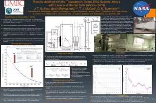
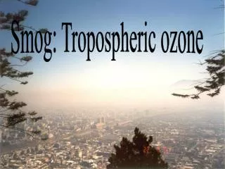
Rise in Tropospheric Ozone overthe20th Century Concentrations of O3 have increased dramatically due to human activity Observations at mountain sites in Europe [Marenco et al., 1994]
Impact of Human Activity on Background O3 O3 Free Troposphere hn greenhouse gas NO NO2 Global Background O3 Direct Intercontinental Transport OH RO2, HO2 Boundary layer (0-2.5 km) RH, CO air pollution (smog) air pollution (smog) O3 NOx Hydrocarbons (RH) O3 NOx Hydrocarbons (RH) CONTINENT 2 CONTINENT 1 OCEAN
“Bottom-up” Emission Inventories Bottom-up emissions E = (fuel burned) x (emission factors) Must extrapolate in space and time using population and economic data Biofuel Emissions are highly uncertain Biomass Burning FossilFuel
How Uncertain are Bottom-up Inventories? EDGAR 1995 CH4 inventory [Olivier, 2002]
Range of uncertainty for 1995 estimate Error based on 15% uncertainty in globally averaged OH How Uncertain are Bottom-up Inventories? [IPCC, 2001] EDGAR 1995 CH4 inventory [Olivier, 2002]
Inverse Modeling Atmospheric“forward” model gives C = kE a priori “bottom-up” estimate Ea sa Monitoring site measures concentration C “top-down” estimate Eese Inverse model E = k-1C • instrument • representativeness • model parameters “observational” error se includes terms from Best “a posteriori” estimate:
Satellite Observations of Tropospheric Chemistry N = NadirL = Limb Increasing spatial resolution
Global Ozone Monitoring Experiment (GOME) • Launched April 1995 • Nadir-viewing solar backscatter instrument (237-794 nm) • Polar sun-synchronous orbit • Complete global coverage in 3 days • Spatial resolution 320x40 km2, three cross-track scenes
GEOS-CHEM Global 3-D Model • Driven by assimilated meteorology from the NASA Data Assimilation Office • Horizontal resolution of 2º latitude x 2.5º longitude • O3-NOx-hydrocarbon chemistry • Emission Inventories: • Isoprene: Global Emission Inventory Activity (GEIA) [Benkovitz et al., 1996] • CO: biofuels (Yevich and Logan,2003), fossil fuels and biomass burning (Duncan et al., 2003)
GOME HCHO Columns for July 1996 2.5 [1016 molec cm-2] 2.0 1.5 1.0 0.5 0 Hot spots reflect high hydrocarbon emissions from fires and biosphere OH CH4 Dominant hydrocarbon sources: CO HCHO Isoprene
GEOS-CHEM Relationship Between HCHO Columns and Isoprene Emissions in N. America NE NW Model HCHO Column [1016 molec cm -2] SE SW Cont. from other sources Isoprene emission [1013 atomC cm-2 s-1] GEOS-CHEMModel, July 1996 (25-50ºN, 65-130ºW) Isoprene lifetime < 1 hour Isoprene emissions correlated with HCHO columns Palmer et al. [2003]
Isoprene Emissions for July 1996 by Scaling of GOME Formaldehyde Columns Use linear relationship between isopreneemissions and HCHO columns from model to map GOME HCHO column to top-down isoprene emissions GOME Top-down emissions provide a better fit to in situobservations of HCHO over US [1012 atom C cm-2 s-1] 0 3 1 5 (official EPA inventory) (a priori inventory in GEOS-CHEM) [Palmer et al., 2003]
The Next Generation: Tropospheric Emission Spectrometer • Will be launched in 2004 • Infrared, high resolution Fourier spectrometer(3.3 - 15.4 mm) • Polar, sun-synchronous orbit • Makes 14.56 orbits per day and repeats its orbit every 16 days • Has 2 viewing modes: a nadir view and a limb view • Spatial resolution of nadir measurement is 8 x 5 km2
OBJECTIVE: Determine whether nadir observations of CO from TES will have enough information to reduce uncertainties in our estimates of continental sources of CO Assume that we know the true sources of CO APPROACH: Use GEOS-CHEM 3-D model to simulate “true” pseudo-atmosphere Sample pseudo-atmosphere along orbit of TES and simulate retrievals of CO Obtain a posteriori sources and errors; How successful are we at finding the true source and reducing the error? Make a priori estimate of CO sources by applying errors to the “true” source Use an optimal estimation inverse method
Inversion Analysis State Vector EUFF NAFF ASFF ASBB AFBB CHEM SABB RWFF RWBB • FF = Fossil Fuel + Biofuel • All sources include contributions from oxidation of VOCs • OH is specified • Use a “tagged CO” method to estimate contribution from each source • Use inverse method to solve for annually-averaged emissions “True” Emissions (Tg/yr) NAFF: 121.3 SABB: 96.5 EUFF: 131.1 RWBB: 98.0 ASFF: 258.3 RWFF: 149.8 ASBB: 96.0 CHEM: 1125.0 AFBB: 193.9 Total = 2270 Tg/yr
Modeled COLevel 13 (6 km) 15 Mar. 2001, 0 GMT North Americanfossil fuel CO tracer
Simulating the TES Data • Sample the synthetic atmosphere along the orbit of TES • Assume that the TES nadir footprint of 8 x 5 km is representative of the entire GEOS-CHEM 2º x 2.5º grid box • We consider data only between the equator and 60ºN • Assume cloud-free conditions CO at 510.9 hPa for March 15, 2001
Generating the Nadir Retrievals of CO The retrieved profile is: ya = a priori profile yt = true profile from GEOS-CHEM A = averaging kernels true profile a priori retrieved
Inversion Methodology • Unlike isoprene, CO has a long lifetime (weeks – months) so transport is important need a more formal inversion analysis • Minimize a maximum a posteriori cost function = retrieved profile x = estimate of the state vector (the CO sources) xa=a priori estimate of the CO sources(generated by perturbing true state) Sa= error covariance of the a priori (assume a priori error of 50%) F(x)= forward model simulation of x Se= error covariance of observations = instrument error + model error + representativeness error
The Forward Model The forward Model (GEOS-CHEM) must account for the verticalsensitivity of TES and the a priori information used in the retrievals H(x) = GEOS-CHEM model ei= Retrieval noise (< 10%, based on spectral noise of instrument) Must add noise to forward model to account for errors in GEOS-CHEM simulation of CO er= representativeness error em= model error
Constructing the Covariance Matrix for the Model Error • The “NMC method” • assume that the difference between successive forecasts, which are valid at the same time, is representative of the forecast error structure Model Level 16 (8 km) CO Mixing Ratio (ppb) • root mean square error based on the difference of 89 pairs of 48-hr and 24-hr forecasts of CO during Feb-April 2001
Characterizing the Model Error • Compare model with observations of CO from TRACE-P and estimate the relative error • Assume mean bias in relative error is due to emission errors • Remove mean bias and assume the residual relative error (RRE) is due to transport • Use RRE to scale forecast error structure Mean forecast error RRE • Representativeness error = 5%, based on sub-grid variability of TRACE-P data
Inversion Results: 4 Days of Pseudo-Data • With unbiased Gaussian error statistics, TES is extremely powerful for constraining continental sources of CO
Conclusions • Current space-based observations provide valuable information to help quantify emissions of O3 precursors • Observations from TES and future high resolution satellite instruments have the potential to significantly enhance our ability to constrain regional source estimates of O3 precursors • Realization of this potential rests on proper error characterization, particularly for the model transport error • Will require an integrated approach – in situ (surface and aircraft) and space-based observations • THE FUTURE: Multi-species chemical data assimilation • Integrate observations from surface sites, aircraft, and satellites (low Earth orbit and geostationary) to construct an optimized 4-D view of the chemical state of the atmosphere
Model Transport Error RMS error b/w model and MOPITT CO column during TRACE-P (Colette Heald) x1018 molec/cm2 Model Level 16 (8 km) RMS error based on the difference of 89 pairs of 48-hr and 24-hr forecasts of CO during TRACE-P CO Mixing Ratio (ppb)
The Forward Model The forward Model (GEOS-CHEM) must account for the verticalsensitivity of TES and the a priori information used in the retrievals H(x) = GEOS-CHEM model G = gain matrix associated with A s = standard deviation of spectral noise Si = G(s2I)GT n = Gaussian white noise with unity variance Gsn= Retrieval noise Must add noise to forward model to account for errors in GEOS-CHEM simulation of CO er= representativeness error em= model error
CO Source Distribution in GEOS-CHEM Fossil Fuels Biofuels Biomass Burning • Other Sources: oxidation of methane and other VOCs • Main sink: reaction with atmospheric OH