Download
1 / 36
360 likes | 506 Vues
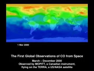
March – December 2000 Observed by MOPITT, a Canadian instrument, flying on the TERRA, a US/NASA satellite. The First Global Observations of CO from Space. Understanding the Hemispheric Transport of Air Pollutants: It’s not just for scientists any more!. An OPAR Brown Bag, 10 April 2013

E N D
March – December 2000Observed by MOPITT, a Canadian instrument, flying on the TERRA, a US/NASA satellite The First Global Observations of CO from Space
Understanding the Hemispheric Transport of Air Pollutants:It’s not just for scientists any more! An OPAR Brown Bag, 10 April 2013 Presented by Terry Keating, PhD • Hemispheric Transport and the Ozone NAAQS • What is TF HTAP and what is it doing? • What is the value-added by TF HTAP for OAR?
Implications of Transport for Air Quality Management • What are the magnitudes of each fraction? • How will each fraction change in the future? • How efficiently can each fraction be mitigated? • What is an appropriate level of responsibility for mitigation in the downwind area? (CAA §179b) • What policies and programs are needed to bring about mitigation of upwind sources? NAAQS “PRB”
Annual 4th Highest Daily Maximum 8-Hour Average Ozone Absent Anthropogenic Emissions from the United States, Canada, and MexicoSimulated by GEOS-Chem for 2006-2008(i.e. North American Background, formerly known as PRB) The last O3 NAAQS review considered a level of this metric between 60 and 70 ppb. Zhang et al (2011) Atmospheric Environment, 45:6769
Seasonal Mean Maximum Daily 8-Hour Average Ozone Simulated by GEOS-Chem “North American Background” (Formerly known as PRB) Canadian & Mexican Influences Influences from Anthropogenic Emissions outside North America From Zhang et al 2011
Asian pollution contribution to high surface O3 events, confounding to attain tighter standard in WUS AM3/C180 total ozone Obs (CASTNet/AQS) AM3/C180 Asian ozone June 21 2010 June 22 2010 Max daily 8-h average Lin et al 2012
The Asian enhancement increases for total O3 in the 70-80 ppb range over Southern California, Arizona 25th Lin et al 2012
What is the TF HTAP? Task Force on Hemispheric Transport of Air Pollution • An expert group established in 2004 by the UNECE Convention on Long-Range Transboundary Air Pollution (LRTAP) • Co-Chaired by the European Commission (Dr. Frank Dentener, Joint Research Centre) & the United States (Dr. Terry Keating, EPA/OAR) • Phase 1: 2005-2010, culminated in first comprehensive assessment of HTAP • Phase 2: 2011-2016, working to improve the resolution of our assessment • www.htap.org
What is the TF HTAP? Red border indicates U.S. participation.
Parties to the Convention on Long-Range Transboundary Air Pollution LRTAP was formed in 1979 under the United Nations Economic Commission for Europe.
Parties to the Convention on Long-Range Transboundary Air Pollution And Other Participants in TF HTAP Approximately 750 individual scientists have taken part in at least one TF HTAP activity since 2005. Less than 10% have received specific funding support from EPA or EC.
HTAP 2010 Findings Can current global models adequately simulate intercontinental transport of ozone? Mediterranean Central Europe > 1km Central Europe < 1km NE USA SW USA SE USA Monthly Mean Surface Ozone (ppb) Japan Mountainous W USA Great Lakes USA • There is a large spread across models. The ensemble mean generally captures observed monthly mean surface O3 but there are notable biases. • Simulation of O3 is generally good in early spring and late fall when intercontinental transport is largest.
HTAP 2010 Findings Do current global models produce similar estimates of intercontinental source-receptor relationships? EU NA EA SA • Source-Receptor Sensitivity Simulations: • Base Year 2001 • Decrease emissions of precursors in each region by 20% • Compare effects of different combinations of precursors • Approximately 30 modeling groups from around the world participated
HTAP 2010 Findings Ozone Source-Receptor Analysis under HTAPchange in monthly mean O3 due to 20% reduction of NOX, VOC, and CO emissions N. American Emissions European Emissions South Asian Emissions East Asian Emissions 24 (+8) models contribute results; 14 models complete full set
HTAP 2010 Findings How has surface O3 changed? How well does this match observations? 1974-2004 trend: Obs 0.15 ppb/yr, Mod 0.13 ppb/yr 1989-2007 trend: Obs 0.17 ppb/yr, Mod -0.03 ppb/yr Wild, et al 2013
HTAP 2010 Findings Role of CH4 in Future O3 Scenarios Linearized results of 6 models: O3 Change in 4 RCP Scenarios CH4, Regional, & Imported Components of O3 Change in “High” Scenario Components of O3 Change in “Low” Scenario CH4 is an important determinant of future O3 levels, potentially offsetting benefits of regional controls.
Current Work Plan Work Plan for 2012-2016 The focus of the Task Force’s work remains on characterizing regional vs. extra-regional influences on air quality and its impacts. While HTAP 2010 presented the significance of intercontinental transport with very coarse resolution, our goal now is to improve the resolution of that picture by linking analyses at the global and regional scale. Overall Objectives of Work Plan • Deliver Policy Relevant Information to the LRTAP Convention, Other Multi-Lateral Forums, and National Governments • Improve Our Scientific Understanding of Air Pollution at the Global to Hemispheric Scale • Build a Common Understanding by Engaging Experts Inside and Outside the LRTAP Convention
Current Work Plan Themes of Cooperative Activities Under TF HTAP 1. Emissions & Projections Policy-Relevant Science Products & Outreach 2. Source/Receptor & Source Apportionment 3. Model/Observation & Process Evaluation 4. Impacts on Health, Ecosystems, & Climate 5. Impact of Climate Change on Pollution 6. Data Network & Analysis Tools > 35 Work Packages identified, each with a volunteer leader.
Current Work Plan Emissions & Projections • 2008 & 2010 Global Emissions Mosaics (WP1.1) • JRC is compiling a new global emissions consistent with regional modeling inventories being used in the United States, Europe, and Asia. • Expecting model ready emissions information by July 1, 2013. HTAPv2
Current Work Plan Emissions & Projections • 2010-2030 Emissions Scenarios (WP1.2) • IIASA is developing 3 benchmark scenarios with explicit air pollution controls: • Current Legislation, No Further Control, Maximum Feasible Reduction • Based on IEA energy projections, OAP has provided input on CH4 emissions • Will serve as basis for discussion about available control strategies
Status of HTAP Efforts Source-Receptor Analyses • Common Specification of Regions in a 2 Tier System Tier 1 = 16 regions Tier 2 = 60 regions
Current Work Program Source-Receptor Analyses • Nesting of Regional Analyses Within Global Analyses • Air Quality Model Evaluation International Initiative (AQMEII) Phase II, covering regional domains in North America and Europe • Led by Christian Hogrefe (ORD) and Stefano Galmarini (JRC) • Model Inter-Comparison Study – Asia Phase III, covering regional domains in Asia • Led by Greg Carmichael (U Iowa), Zifa Wang (Chinese Academy of Sciences), and Hajime Akimoto (Asian Center for Air Pollution Research, Japan) • Comparison of Source Apportionment and Sensitivity Techniques • Led by Daven Henze (U Colorado) • Emission Perturbation Analysis • Adjoint Modeling • Pollutant Tagging • Artificial Tracers
Current Work Program Work Flow and Timeline 2008-2010 Emissions Deliver July 1 2010-2030 Scenarios Deliver July? Start July Global Base Modeling Regional Base Modeling Start Sept Global – Regional Perturbations Model-Obs Analysis Start Oct Workshop? Method Comparison Start Oct-Jan Start Jan 2014 Parameterization Start Oct-Jan Impact Assessments Impacts of Mitigation Start Jun 2014
Status of HTAP Efforts Model-Observation Evaluations Case Study on Import to Western North America (WP3.2) Led by Owen Cooper (NOAA)
Status of HTAP Efforts Impact Assessment Methods • Human Health Effects • Led by Jason West (UNC) with Susan Anenberg (EPA/OAR/OAQPS) • Building upon the Global Burden of Disease Study • Ecosystem Effects • Led by Lisa Emberson (SEI-York) • Building upon the work of LRTAP Working Group on Effects • Climate Effects • Led by Bill Collins (Reading Univ, UK) • Moving beyond radiative forcing and global temperature changes • Proposed Workshop on Impact Assessment Methods • Pune, India? • Potential to link to Male Declaration, ABC-Asia, CCAC, and other UNEP activities
Why TF HTAP? Value-Added of TF HTAP for OAR • Filling Gaps in U.S. Program • E.g., global emissions inventories and air pollution control scenarios • Value of the Model Ensemble and Community Effort • A single model will give you an answer, but you don’t know how good it is. • Approach and results have gone through some peer vetting in an open process. • Ability to Focus Research on Policy-Relevant Questions • The science community wants to be useful to the policy community. • Products have many uses at both the global and regional scale. • E.g., Arctic transport, data networking, observational data collections • Low Investment, High Yield • 10:1 payoff for meeting costs. 3:1 leveraging for infrastructure investments. • Building relationships and technical capacities. • Country to Country, Science to Policy, Scientist to Scientist • Creating a Foundation for Decision-making and Action
Additional Slides on O3 Trends Visit www.htap.org for more information.
Summer 1990-2010 Rural ozone trends significant increase insignificant increase significant decrease insignificant decrease Cooper, O. R., et al. (2012), Long-term ozone trends at rural ozone monitoring sites across the United States, 1990–2010, J. Geophys. Res., 117, D22307
Spring 1990-2010 Rural ozone trends significant increase insignificant increase significant decrease insignificant decrease Cooper, O. R., et al. (2012), Long-term ozone trends at rural ozone monitoring sites across the United States, 1990–2010, J. Geophys. Res., 117, D22307
Free tropospheric ozone trend above western North America in April & May 1984-2011 95% 67 % 50% 33% 5 % All available data above western North America, regardless of transport history, including observations by ballons (sondes) and commercial and research aircraft. All measurements were made between 3.0 – 8.0 km above sea level during April-May. Ozone above the surface has increased by 29% from 1984-2011. Cooper, O. R., et al. (2012), Long-term ozone trends at rural ozone monitoring sites across the United States, 1990–2010, J. Geophys. Res., 117, D22307
Surface ozone trends, beginning 1990-1999 and ending 2000-2010. All trends are from the peer-reviewed literature. significant increase insignificant increase significant decrease insignificant decrease From Owen Cooper (NOAA) for IPCC AR5
Average NO2 Column From Space April-May 1996-1998 (GOME) From Cooper, 2013
Average NO2 Column From Space April-May 2009-2011 (SCHIAMACHY) Seasonal Average NO2 Column (Mar, Apr, May,Jun, Jul, Aug, Sep, Oct) with Annual Fossil Fuel CO2 Emissions (in black) from 1995 to 2011 From Cooper, 2013