Chapter 3 working with combinational logic
Chapter 3 working with combinational logic. Working with combinational logic. Simplification two-level simplification exploiting don’t cares algorithm for simplification Logic realization two-level logic and canonical forms realized with NANDs and NORs

Chapter 3 working with combinational logic
E N D
Presentation Transcript
Working with combinational logic • Simplification • two-level simplification • exploiting don’t cares • algorithm for simplification • Logic realization • two-level logic and canonical forms realized with NANDs and NORs • multi-level logic, converting between ANDs and ORs • Time behavior • Hardware description languages The first important topic here is formalizing the process of boolean minimization. In the last chapter, we illustrated how logic functions (or its expressions) can be simplified by boolean cubes or K-maps. Here we will look at a systematic or algorithmic approach.
A B C D LT EQ GT 0 0 0 0 0 1 0 0 1 1 0 0 1 0 1 0 0 1 1 1 0 0 0 1 0 0 0 0 1 0 1 0 1 0 1 0 1 0 0 1 1 1 0 0 1 0 0 0 0 0 1 0 1 0 0 1 1 0 0 1 0 1 1 1 0 0 1 1 0 0 0 0 1 0 1 0 0 1 1 0 0 0 1 1 1 0 1 0 A N1 LTEQGT A B < C DA B = C DA B > C D B C N2 D block diagram and truth table Design example: two-bit comparator we'll need a 4-variable Karnaugh map for each of the 3 output functions Before going into the formal minimization process, let’s look at some examples. The first example compares two numbers, each of which is two bits long, N1 is AB and N2 is CD, where A and C are most significant bits (MSBs) while B and D are least significant bits (LSBs).
A A 0 0 0 0 0 0 0 0 1 0 0 1 0 0 1 0 A' B' D + A' C + B' C D D D A' B' C' D' + A' B C' D + A B C D + A B' C D’ 0 1 0 0 1 0 0 1 0 0 0 0 1 1 1 1 B C' D' + A C' + A B D' C C B B Design example: two-bit comparator (cont’d) A 1 1 1 1 0 1 0 0 D 0 0 1 0 0 0 0 0 C B K-map for LT K-map for EQ K-map for GT LT = EQ = GT = = (A xnor C) • (B xnor D) LT and GT are similar (flip A/C and B/D) EQ = (AC +A’C’)BD + (AC+A’C’)B’D’=(AC+A’C’)(BD+B’D’)
A B C D EQ EQ Design example: two-bit comparator (cont’d) two alternative implementations of EQ with and without XOR XNOR is implemented with at least 3 simple gates
A1 A2B1 B2 P1 P2P4 P8 Design example: 2x2-bit multiplier A2 A1 B2 B1 P8 P4 P2 P1 0 0 0 0 0 0 0 0 0 1 0 0 0 0 1 0 0 0 0 0 1 1 0 0 0 0 0 1 0 0 0 0 0 0 0 1 0 0 0 1 1 0 0 0 1 0 1 1 0 0 1 1 1 0 0 0 0 0 0 0 0 1 0 0 1 0 1 0 0 1 0 0 1 1 0 1 1 0 1 1 0 0 0 0 0 0 0 1 0 0 1 1 1 0 0 1 1 0 1 1 1 0 0 1 block diagram and truth table 4-variable K-map for each of the 4 output functions This is a 2bit-by-2bit multiplier that generates 4 bit output (whose MSB is P8 and LSB is P1). Note that A2 and B2 are MSBs. P? labels in output wires stand for product.
A2 A2 0 0 0 0 0 0 0 0 0 0 0 0 0 0 0 0 B1 B1 1 0 0 0 0 1 1 1 0 0 0 0 0 0 0 0 B2 B2 A1 A1 A2 A2 0 0 1 1 0 0 1 0 0 0 0 0 0 0 0 1 B1 B1 0 1 1 0 1 0 0 0 0 1 0 1 0 1 0 0 B2 B2 A1 A1 Design example: 2x2-bit multiplier (cont’d) K-map for P4 K-map for P8 P4 = A2B2B1' + A2A1'B2 P8 = A2A1B2B1 K-map for P2 K-map for P1 P1 = A1B1 P2 = A2'A1B2 + A1B2B1' + A2B2'B1 + A2A1'B1
I1 I2I4 I8 O1 O2O4 O8 Design example: BCD increment by 1 I8 I4 I2 I1 O8 O4 O2 O10 0 0 0 0 0 0 1 0 0 0 1 0 0 1 0 0 0 1 0 0 0 1 1 0 0 1 1 0 1 0 0 0 1 0 0 0 1 0 1 0 1 0 1 0 1 1 0 0 1 1 0 0 1 1 1 0 1 1 1 1 0 0 0 1 0 0 0 1 0 0 1 1 0 0 1 0 0 0 0 1 0 1 0 X X X X 1 0 1 1 X X X X 1 1 0 0 X X X X 1 1 0 1 X X X X 1 1 1 0 X X X X 1 1 1 1 X X X X block diagram and truth table 4-variable K-map for each of the 4 output functions
I8 I8 I8 I8 X 0 X 0 X 1 X 0 X 0 X 0 X 1 X 0 1 1 0 0 0 0 0 0 0 0 1 1 0 1 0 1 I1 I1 I1 I1 O8 = I4 I2 I1 + I8 I1' O4 = I4 I2' + I4 I1' + I4’ I2 I1O2 = I8’ I2’ I1 + I2 I1' O1 = I1' X X X X X X X X X X X X X X X X 0 0 1 1 1 0 0 1 0 1 0 0 0 0 1 1 I2 I2 I2 I2 I4 I4 I4 I4 Design example: BCD increment by 1 (cont’d) O8 O4 O2 O1 In O8, we will interpret a don’t care (DC) term as 1 if it helps to minimize the number of literals for the elements of the ON-set. The other DC terms will be treated as 0. To minimize the number of literals, we have to find out the maximum size subcube.
Definition of terms for two-level simplification • Implicant • single element of ON-set or DC-set or any group of these elements that can be combined to form a subcube (or an adjacent group) • Prime implicant (PI) • implicant that can't be combined with another to form a larger subcube • Essential prime implicant • prime implicant is essential if it alone covers an element of ON-set • will participate in ALL possible covers of the ON-set • DC-set used to form prime implicants but not to make implicant essential • Objective: • grow implicant into prime implicants(to minimize literals per term) • cover the ON-set with as few prime implicants as possible(to minimize number of product terms) So far we have examined a few examples of logic design simplification From now on, we will try to perform simplification in a systematic or algorithmic way. To do so, we first have to define some terminologies.
A A 6 prime implicants: A'B'D, BC', AC, A'C'D, AB, B'CD 1 0 1 0 1 0 1 0 0 0 1 1 0 X 1 1 D D essential 1 1 1 1 1 1 0 0 1 0 0 0 0 1 0 1 C C B B 5 prime implicants: BD, ABC', ACD, A'BC, A'C'D essential Examples to illustrate terms minimum cover: AC + BC' + A'B'D minimum cover: 4 essential implicants First of all, we have to find out all the possible prime implicants. Then we first transform the essential prime implicants to boolean expressions. Then we will try to find the minimum set of prime implicants to cover the entire on-set, called minimum cover.
Algorithm for two-level simplification • Algorithm: minimum sum-of-products expression from a Karnaugh map • Step 1: choose an element of the ON-set • Step 2: find "maximal" groupings of 1s and Xs adjacent to that element • consider top/bottom row, left/right column, and corner adjacencies • this forms prime implicants (number of elements always a power of 2) • Repeat Steps 1 and 2 to find all prime implicants • Step 3: revisit the 1s in the K-map • if covered by single prime implicant, it is essential, and participates in final cover • 1s covered by essential prime implicant do not need to be revisited • Step 4: if there remain 1s not covered by essential prime implicants • select the smallest number of prime implicants that cover the remaining 1s
A A A A A A A 0 1 1 1 0 1 1 1 0 1 1 1 0 1 1 1 0 1 1 1 0 1 1 1 0 1 1 1 X 1 0 1 X 1 0 1 X 1 0 1 X 1 0 1 X 1 0 1 X 1 0 1 X 1 0 1 D D D D D D D X 0 0 1 X 0 0 1 X 0 0 1 X 0 0 1 X 0 0 1 X 0 0 1 X 0 0 1 0 X 0 1 0 X 0 1 0 X 0 1 0 X 0 1 0 X 0 1 0 X 0 1 0 X 0 1 C C C C C C C B B B B B B B 2 primes around A'BC'D' 2 primes around ABC'D 3 primes around AB'C'D' 2 essential primes minimum cover (3 primes) Algorithm for two-level simplification (example) For all 1s, check the PIs that include the 1. The PIs should be considered for all the 1s and DCs around that can be united. Then we first choose essential PIs and then find out the minimum cover, the minimum number of PIs that cover the remaining 1s.
A A X 0 X 1 X 0 X 1 X 0 0 1 X 0 0 1 D D X 0 1 1 X 0 1 1 0 X X 1 0 X X 1 C C CD’ BC BD AB AC’D B B Activity • List all prime implicants for the following K-map: • Which are essential prime implicants? • What is the minimum cover? CD’ BD AC’D CD’ BD AC’D Let’s start with prime implicants. Among PIs, check which are essential. Finally, we should find out the minimum cover, which is the minimum number of PIs that cover all the elements of the ON-set (including essential PIs)
Implementations of two-level logic A B C • Sum-of-products • AND gates to form product terms (minterms) • OR gate to form sum • Product-of-sums • OR gates to form sum terms (maxterms) • AND gates to form product In this section, we will focus on how to implementlogic networks with NAND or NOR gates. Again there are two kinds of canonical forms: S-O-P and P-O-S. A small circle is an inverter.
Two-level logic using NAND gates A B C A B C • Replace minterm AND gates with NAND gates • Place compensating inversion at inputs of OR gate NAND/NOR gates requires less CMOS TRs than AND/OR gates. So we want to change AND/OR gates into NAND gates only (or NOR gates only) The simplest way is to insert double inverters between AND and OR gates. Then what happens is that AND becomes NAND just by placing bubbles. How about the OR gate?
Two-level logic using NAND gates (cont’d) • OR gate with inverted inputs is a NAND gate • de Morgan’s: A’ + B’ = (A • B)’ • Two-level NAND-NAND network • inverted inputs are not counted • in a typical circuit, inversion is done once and signal distributed Recall de Morgan’s Law. When inverters are passing through a gate, the gate should be changed from OR to AND and vice versa.
Two-level logic using NOR gates • Replace maxterm OR gates with NOR gates • Place compensating inversion at inputs of AND gate In the case of P-O-S forms, the same technique is used; however, this time, the NOR gate is the results of conversion. Again, we insert two bubbles between OR and AND gates and push those bubbles in the opposite directions.
Two-level logic using NOR gates (cont’d) • AND gate with inverted inputs is a NOR gate • de Morgan’s: A’ • B’ = (A + B)’ • Two-level NOR-NOR network • inverted inputs are not counted • in a typical circuit, inversion is done once and signal distributed Using de Morgan’s theorem again, the AND gate with inverted inputs is transformed into the NOR gate as shown in the above.
Two-level logic using NAND and NOR gates • NAND-NAND and NOR-NOR networks • de Morgan’s law: (A + B)’ = A’ • B’ (A • B)’ = A’ + B’ • written differently: A + B = (A’ • B’)’ (A • B) = (A’ + B’)’ • In other words –– • OR is the same as NAND with complemented inputs • AND is the same as NOR with complemented inputs • NAND is the same as OR with complemented inputs • NOR is the same as AND with complemented inputs This slide summarizes what I explained about conversion from AND-OR combination to either NAND or NOR gates. All the conversions are just variations of de morgan’s theorem.
A A NAND B B Z Z NAND C C NAND D D Conversion between forms • Convert from networks of ANDs and ORs to networks of NANDs and NORs • introduce appropriate inversions ("bubbles") • Each introduced "bubble" must be matched by a corresponding "bubble" • conservation of inversions • do not alter logic function • Example: AND/OR to NAND/NAND Again, inverters inserted between gates are called bubbles. In order to make no changes in the logic function, the bubbles are always paired.
A A NAND B B Z Z NAND C C NAND D D Conversion between forms (cont’d) • Example: verify equivalence of two forms Z = [ (A • B)’ • (C • D)’ ]’ = [ (A’ + B’) • (C’ + D’) ]’ = [ (A’ + B’)’ + (C’ + D’)’ ] = (A • B) + (C • D) Let’s verify the conversion rule by boolean expressions and boolean theorems
A \A B NOR Z \B C D Z NOR A NOR \C NOR B \D Z Step 2 C NOR D Conversion between forms (cont’d) • Example: map AND/OR network to NOR/NOR network Step 1 conserve "bubbles" conserve "bubbles" When an input variable, say A, is complemented, it is denoted by \A When a S-o-P canonical form is converted to NOR networks, we have to insert two bubbles at the input stage. And the same thing happens at the output stage.
A B Z C D \ A NOR \ B NOR Z \ C NOR \ D Conversion between forms (cont’d) • Example: verify equivalence of two forms Z = { [ (A’ + B’)’ + (C’ + D’)’ ]’ }’ = { (A’ + B’) • (C’ + D’) }’ = (A’ + B’)’ + (C’ + D’)’ = (A • B) + (C • D) This is the boolean logic proof of the conversion in the previous slide.
Multi-level logic • x = A D F + A E F + B D F + B E F + C D F + C E F + G • reduced sum-of-products form – already simplified • 6 x 3-input AND gates + 1 x 7-input OR gate (that may not even exist!) • 25 wires (19 literals plus 6 internal wires) • x = (A + B + C) (D + E) F + G • factored form – not written as two-level S-o-P • 1 x 3-input OR gate, 2 x 2-input OR gates, 1 x 3-input AND gate • 10 wires (7 literals plus 3 internal wires) A BC DEFG X If there are common parts in a canonical form, it may be better to use multi-level logic to reduce the number of literals and gates at the cost of delay. Again tradeoff between delay and gate count
C D F B A original AND-OR network B \C C D introduction and conservation of bubbles F B A B \C C D F \B A redrawn in terms of conventional NAND gates B \C Conversion of multi-level logic to NAND gates Level 1 Level 2 Level 3 Level 4 • F = A (B + C D) + B C’ Normally when we add two bubbles in a wire, two levels are converted to NAND gates. Here we add two bubbles between AND and OR gates.
C D F B A B original AND-OR network \C C D F B A introduction and conservation of bubbles B \C Conversion of multi-level logic to NORs Level 1 Level 2 Level 3 Level 4 • F = A (B + C D) + B C’ . \ C \ D redrawn in terms of conventional NOR gates F B \ A \ B C Here we add bubbles in different position to use NOR gates. Note that the final inverter is implemented by NOR!
A A B B F F C C X X D D add double bubbles to invert all inputs of OR gate original circuit A A X B F C X B F \ D C \ X \ D add double bubbles to invert output of AND gate insert inverters to eliminate double bubbles on a wire Conversion between forms • Example This slide illustrates how we can convert a combination of AND and OR gates into NAND and NOT gates. As mentioned before, NOT gates can be replaced by NAND gates by splitting the input.
possible implementation logical concept A A B B Z Z C C D D Invert AND NAND NAND OR Invert & & 2x2 AOI gate symbol 3x2 AOI gate symbol + + & & AND-OR-Invert (AOI) gates • AOI function: three stages of logic — AND, OR, Invert • multiple gates "packaged" as a single circuit block Here is a special case of AND-OR-Inverter gates, which is a popular combination in a logic package. The reason it becomes a popular combination is that it can be implemented compactly with CMOS TRs.
AOI example • Why AOI is more compact than NAND or NOR? out = [ab+c]’: invert symbol circuit or and
& A’ + & B’ F A B Conversion to AOI forms • General procedure to place in AOI form • compute the complement of the function in sum-of-products form • by grouping the 0s in the Karnaugh map • Example: XOR implementation • A xor B = A’ B + A B’ • AOI form: • F = (A’ B’ + A B)’ Let’s take an example to use AOI to implement a logic function. Suppose we have to implement a XOR function. F = AB’+A’B. first of all, we consider F’ (note that there is an inverter at the end of AOI). F’ = AB+A’B’. So we implement F’ in the SOP form.
Summary for multi-level logic • Advantages • circuits may be smaller • gates have smaller fan-in • Disadvantages • circuits will be slower • more difficult to design • tools for optimization are not as good as for two-level • analysis is more complex Multi-level logic design can reduce the number of gates or at least the number of fan-ins of gates. However, optimization is more complex.
Time behavior of combinational networks • Waveforms • visualization of values carried on signal wires over time • useful in explaining sequences of events (changes in value) • Simulation tools are used to create these waveforms • input to the simulator includes gates and their connections • input stimulus, that is, input signal waveforms • Some terms • gate delay — time for change at input to cause change at output • min delay – typical/nominal delay – max delay • careful designers design for the worst case • rise time — time for output to transition from low to high voltage • fall time — time for output to transition from high to low voltage • pulse width — time that an output stays high or stays low between changes The next topic of this chapter is the behavior of combinational logic as time goes by. The waveform of a system can be simulated by a tool considering gates and their connections. The output of the system is triggered by the input stimulus.
A B C D F Momentary changes in outputs • Can be useful — pulse shaping circuits • Can be a problem — incorrect circuit operation (glitches/hazards) • Example: pulse shaping circuit • A’ • A = 0 • delays matter D remains high for three gate delays after A changes from low to high F is not always 0 pulse 3 gate-delays wide Let’s see how a waveform changes over time in this case. Here, each gate is assumed to incur 10 time unit delay. This time-varying behavior is utilized to make a periodic pulse.
+ resistor A B open switch C D Oscillatory behavior • Another pulse shaping circuit close switch initially undefined open switch Assume that each gate delay is 10 time units. Here, the output of NAND is feedback to its input with a couple of inverters. Let’s look at the waveform of B. what does it look like?
Hardware description languages (HDLs) • Describe hardware at varying levels of abstraction • Structural description • textual replacement for schematic • hierarchical composition of modules from primitives • Behavioral/functional description • describe what module does, not how • synthesis generates circuit for module • Simulation semantics This is the last topic of chapter 3. So far, we rely on boolean expressions and schematic drawings to describe logic functions. However, as a logic function gets complicated, it will become extremely hard to write and understand the logic system. Hierarchy can help to mitigate this problem; but it is not enough. HDLs are proposed to deal with this problem. Using HDLs, we can describe any complicated logic system. Moreover, the languages can be executed, they run like s/w. A program emulates the behavior of the designed system as faithfully as possible. It radically reduces the time to design a system
HDLs • Abel (circa 1983) - developed by Data-I/O • targeted to programmable logic devices • not good for much more than state machines • ISP (circa 1977) - research project at CMU • simulation, but no synthesis • Verilog (circa 1985) - developed by Gateway (absorbed by Cadence) • similar to Pascal and C • delay is only interaction with simulator • fairly efficient and easy to write • IEEE standard • VHDL (circa 1987) - DoD sponsored standard • similar to Ada (emphasis on re-use and maintainability) • simulation semantics visible • very general but verbose • IEEE standard V: very high speed IC Verilog and VHDL are the most popular HDLs. This course does not aim to cover HDLs in-depth.
Verilog • Supports structural and behavioral descriptions • Structural • explicit structure of the circuit • e.g., each logic gate instantiated and connected to others • Behavioral • program describes input/output behavior of circuit • many structural implementations could have same behavior • e.g., different implementation of one Boolean function • We’ll mostly be using behavioral Verilog • rely on schematic when we want structural descriptions There are two approaches in describing the system (or its modules). A structural description specifies the system textually in terms of logic gates A behavioral description can handle more dynamic properties of the system, which is the focus in the textbook.
Structural model module xor_gate (out, a, b); input a, b; output out; wire abar, bbar, t1, t2; inverter invA (abar, a); inverter invB (bbar, b); and_gate and1 (t1, a, bbar); and_gate and2 (t2, b, abar); or_gate or1 (out, t1, t2); endmodule and1 a invA or1 t1 bbar out t2 abar invB b and2 Here is one example of a structural model description. Wire is used to declare internal variables, which correspond to internal wires. Three types of gates are already included in the Verilog language, just like library functions.
Simple behavioral model • Continuous assignment module xor_gate (out, a, b); input a, b; output out; reg out; assign #6 out = a ^ b; endmodule simulation register - keeps track ofvalue of signal delay from input changeto output change Here is one example of a behavioral model description. reg is used to declare “out,” which should be kept track of by a register whenever there is a change. assign means that “out” should be evaluated again whenever there is a change in “a” or “b”. ^ is x-or in Verilog. #6 means it takes 6 time units while the input change is propagated to the output value
Simple behavioral model module xor_gate (out, a, b); input a, b; output out; reg out; always @(a or b) begin #6 out = a ^ b; end endmodule • always block specifies when block is executed ie. triggered by which signals The always block is another expression which is equivalent to the assign sentence in the previous slide. @ sign indicates that this block should be evaluated whenever there is a change in a or b. The list after @ is called the sensitivity list.
Driving a simulation through a “testbench” module testbench (x, y); output x, y; reg [1:0] cnt; initial begin cnt = 0; repeat (4) begin #10 cnt = cnt + 1; $display ("@ time=%d, x=%b, y=%b, cnt=%b", $time, x, y, cnt); end #10 $finish; end assign x = cnt[1]; assign y = cnt[0];endmodule 2-bit vector initial block executed only once at startof simulation print to a console directive to stop simulation A testbench is the module that drives the designed system by triggering input stimuli. The repeat block will be iterated 4 times. This means x, y are the input variables of the system. The role of the initial block is to schedule the change of input variables.
Complete simulation • Instantiate stimulus component and device to test in a schematic p.144 a z x test-bench y b If we combine the testbench module with the X-or module, the Verilog progrma will do the function as shown here.
HDLs vs. programming languages (PLs) • Program structure • instantiation of multiple components of the same type • specify interconnections between modules via schematic • hierarchy of modules • Assignment • continuous assignment (logic always computes) • propagation delay (computation takes time) • timing of signals is important (when does computation have its effect) • Data structures • size explicitly spelled out - no dynamic structures • no pointers • Parallelism • hardware is naturally parallel (must support multiple threads) • assignments can occur in parallel (not just sequentially) Even though a hierarchical structure is common on HDLs and PLs, there are some fundamental differences between HDLs and PLs. For example, continuous assignment and propagation delay are not typically supported in PLs.
HDLs and combinational logic • Modules - specification of inputs, outputs, bidirectional, and internal signals • Continuous assignment - a gate’s output is a function of its inputs at all times (doesn’t need to wait to be "called") • Propagation delay- concept of time and delay in input affecting gate output • Composition - connecting modules together with wires • Hierarchy - modules encapsulate functional blocks HDLs can describe every aspect of combinational logic systems.
Working with combinational logic summary • Design problems • filling in truth tables • incompletely specified functions • simplifying two-level logic • Realizing two-level logic • NAND and NOR networks • networks of Boolean functions and their time behavior • Time behavior • Hardware description languages • Later • combinational logic technologies • more design case studies