Graduate Course: Advanced Remote Sensing Data Analysis and Application
250 likes | 385 Vues
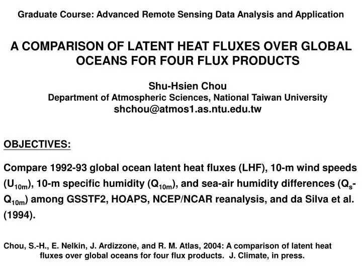
Graduate Course: Advanced Remote Sensing Data Analysis and Application A COMPARISON OF LATENT HEAT FLUXES OVER GLOBAL OCEANS FOR FOUR FLUX PRODUCTS Shu-Hsien Chou Department of Atmospheric Sciences, National Taiwan University shchou@atmos1.as.ntu.edu.tw. OBJECTIVES:

Graduate Course: Advanced Remote Sensing Data Analysis and Application
E N D
Presentation Transcript
Graduate Course: Advanced Remote Sensing Data Analysis and Application A COMPARISON OF LATENT HEAT FLUXES OVER GLOBAL OCEANS FOR FOUR FLUX PRODUCTSShu-Hsien ChouDepartment of Atmospheric Sciences, National Taiwan Universityshchou@atmos1.as.ntu.edu.tw OBJECTIVES: Compare 1992-93 global ocean latent heat fluxes (LHF), 10-m wind speeds (U10m), 10-m specific humidity (Q10m), and sea-air humidity differences (Qs-Q10m) among GSSTF2, HOAPS, NCEP/NCAR reanalysis, and da Silva et al. (1994). Chou, S.-H., E. Nelkin, J. Ardizzone, and R. M. Atlas, 2004: A comparison of latent heat fluxes over global oceans for four flux products. J. Climate, in press.
Latent Heat Flux (FLH) • FLH = r Lv CE (U–Us) (Qs–Q) • CE depends on U, (qs–q), and (Qs–Q)
GSSTF2 BULK FLUX MODEL: (Chou 1993; Chou et al. 2003) * CD, CH, and CE depend on U, (qs–q), and (Qs–Q) (Monin-Obukhov similarity theory) CD = k2/[ln(Z/ZO) – yu(Z/L)]2 CE = CD1/2 k/[ln(Z/ZOq) – yq(Z/L)] Zo = 0.0144 u*2/g + 0.11u/u*(momentum roughness length) Zoq = u/u*[a2(ZOu*/u)b2] (humidity roughness length)
GSSTF2 BULK FLUX MODEL: (Chou 1993; Chou et al. 2003) Wind Stress t = ru*2 Sensible Heat Flux FSH = – r Cp u* q* Latent Heat Flux FLH = – r Lv u* q* Flux –Profile Relationship in Atmospheric Surface Layer: (U – Us)/u* = [ln(Z/Zo) – yu(Z/L)]/k (q – qs)/q* = [ln(Z/ZoT) – yT(Z/L)]/k (Q – Qs)/q* = [ln(Z/Zoq) – yq(Z/L)]/k y =∫(1 – f) d ln(Z/L), L = qv u*2/(g k qv*) Fu= (1 – 16 Z/L)-0.25 , fT= fq= (1 – 16 Z/L )-0.5 (unstable) fu= fT= fq = 1 + 7 Z/L (stable), k = 0.40
Outlines: • Motivation • What are four flux products compared • Validation of latent heat flux (LHF), surface wind speed (Ua), and surface air humidity (Qa) for GSSTF2 • Comparison of U10m • Comparison of Q10m • Comparison of Qs-Q10m • Comparison of LHF
Motivations: • Ocean surface LHF plays an essential role in global energy and water cycle variability • LHF is derived from surface winds, surface air humidity and temperature, and SST using various bulk flux algorithms • All input parameters may have a large uncertainty in reanalyses, satellite retrievals, and COADS. • There is no "ground truth" for global LHF fields; thus it is important to conduct intercomparison studies to assess sources of errors for various global LHF products. • The study can identify the strengths and weaknesses of various LHF products, and provide important information for improving atmospheric GCMs and satellite retrievals.
Four Flux Data Sets Compared: • GSSTF2: 1o daily turbulent fluxes for 1987-2000 from SSM/I (Chou et al. 2003) • HOAPS: Hamburg Ocean Atmosphere Parameters and Fluxes from Satellite Data; derived 0.5o daily surface fluxes for 1987–1998 from SSM/I (version I; Grassl et al. 2000) • NCEP: NCEP/NCAR reanalysis (Kalnay et al. 1996) • Da Silva: 1o monthly climatology (1945-89) and anomalies (up to 1993) of fluxes of heat, momentum, and fresh water along with input parameters; derived from Comprehensive Ocean-Atmosphere Data Set (COADS) mainly from merchant ships (da Silva et al. 1994)
1913-hourly fluxes calculated from ship data using GSSTF2 bulk flux model vs observed latent heat fluxes determined by covariance method of 10 field experiments. C: COARE F: FASTEX X: other experiments
GSSTF2 daily (a) latent heat fluxes, (b) surface winds, and (c) surface air specific humidity vs those of nine field experiments. C: COARE F: FASTEX X: other experiments
The 10-m wind speed averaged over 1992–93 for (a) GSSTF2, and differences of (b) HOAPS, (c) NCEP, and (d) da Silva from GSSTF2.
Standard deviations of differences (left) and temporal cross correlation (right) of monthly 10-m wind speeds between GSSTF2 and each of (a, b) HOAPS, (c, d) NCEP, and (e, f) da Silva during 1992–93.
The 10-m specific humidity averaged over 1992–93 for (a) GSSTF2, and differences of (b) HOAPS, (c) NCEP, and (d) da Silva from GSSTF2.
The sea-air humidity differences averaged over 1992–93 for (a) GSSTF2, and differences of (b) HOAPS, (c) NCEP, and (d) da Silva from GSSTF2.
Standard deviations of differences (left) and temporal cross correlation (right) of monthly 10-m specific humidity between GSSTF2 and each of (a, b) HOAPS, (c, d) NCEP, and (e, f) da Silva during 1992–93.
The latent heat fluxes averaged over 1992–93 for (a) GSSTF2, and differences of (b) HOAPS, (c) NCEP, and (d) da Silva from GSSTF2.
Standard deviations of differences (left) and temporal cross correlation (right) of monthly latent heat fluxes between GSSTF2 and each of (a, b) HOAPS, (c, d) NCEP, and (e, f) da Silva during 1992–93.
CONCLUSIONS: • GSSTF2 daily LHF and input parameters compare reasonably well with those of nine collocated field experiments during 1991-1999. • Comparisons with high quality research ship data suggest that 1992-93 mean GSSTF2 LHF, surface air humidity, and winds are more realistic than the other three flux datasets examined (HOAPS, NCEP, and da Silva). • Over tropical oceans (20oS-20oN), HOAPS LHF is significantly smaller than GSSTF2 by ~31% (37 W m-2), due to weaker U10m (~1.1 m s-1) and smaller QS–Q10m (~0.7 g kg-1), which is due to significant larger Q10m (1.1 g kg-1).
CONCLUSIONS (continued): 4. In equatorial Indian Ocean, SPCZ, ITCZ, Kuroshio and Gulf Stream, and subtropics, NCEP LHF is larger than GSSTF2 (with maximum difference up to 40 W m-2), due to effects of larger NCEP QS–Q10m and CE overcompensating effect of smaller U10m on LHF. For the rest of the oceans, NCEP LHF is smaller than GSSTF2, with the maximum difference of ~60 W m-2 located in dry tongue and trade wind region of eastern South Pacific due to smaller QS–Q10m and U10m. 5. LHF difference of da Silva from GSSTF2 has small-scale structures, with some nearby extreme large positive and negative LHF difference centers located in the data sparse regions; da Silva also has extremely low temporal correlation and large differences with GSSTF2 for all variables in the southern extratropics, indicating da Silva hardly produces a realistic variability in these variables. 6. Temporal correlation is higher in the northern extratropics than in the south for all variables, with the contrast being especially large for da Silva due to more missing ship observations in the south.