Creating Picture Graphs in Excel: Step-by-Step Guide
Learn how to create visually appealing picture graphs in Excel using easy steps. From inputting data to formatting points, this tutorial covers it all to enhance your charts. Perfect for beginners!


Creating Picture Graphs in Excel: Step-by-Step Guide
E N D
Presentation Transcript
Creating Picture Graphs in Excel June 17, 2010
Picture Graphs Excel Data • Open Excel • Type in the data
Picture Graphs The Chart, Part 1 • Highlight the data • Select the Insert Ribbon, then the ‘Column’ button • Click on the 3-D Cylinder chart button Insert Ribbon Column 3-D Cylinder
Picture Graphs The Chart, Part 2 • The chart, inserted
Picture Graphs Move the Chart • Click the ‘Move Chart’ button at the upper right • Select ‘New sheet’, then name it ‘Picture Chart’ Picture Chart New Sheet
Picture Graphs The Chart in a New Tab • Here’s how it looks
Picture Graphs Format the Data Point, Part 1 • Select the Chart Tools Layout Tab • Click the desired data point. You may have to click again to get just the one • Click the ‘Format Selection’ button (or, right-click the selected column) Layout Format Selection
Picture Graphs Format the Data Point, Part 2 • Under the ‘Series Options’ tab, slide the ‘Gap Width’ pointer to the • left, from 150% down to 38% 150% 38%
Picture Graphs Format the Data Point, Part 3 • This is the effect of decreasing the space between the columns
Picture Graphs Format the Data Point, Part 4 • Select the ‘Fill’ tab, then Click ‘Picture or texture fill’ • Click the Insert From: File’ button, pick a picture, and select ‘Stretch’ Picture or Texture Fill Insert From: File
Picture Graphs Format the Data Point, Part 5 • The effect of Stack Stack
Picture Graphs Format the Data Point, Part 6 • The effect of Stack and Scale with 2 2