Download
1 / 24
300 likes | 627 Vues
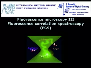
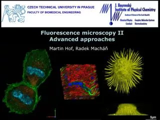
CZECH TECHNICAL UNIVERSITY IN PRAGUE FACULTY OF BIOMEDICAL ENGINEERING . Fluorescence microscopy II Advanced approaches. Martin Hof, Radek Macháň. Microscope resolution :. The lateral resolution of an optical microscope d :.

E N D
CZECH TECHNICAL UNIVERSITY IN PRAGUE FACULTY OF BIOMEDICAL ENGINEERING Fluorescence microscopy IIAdvanced approaches Martin Hof, Radek Macháň
Microscope resolution: The lateral resolution of an optical microscope d: The axial resolution (in the direction of optical axis) dz: Sufficient contrast is necessary for full utilization of the available resolution However fluorescence from planes below and above focus also contributes to signal blurred image, decreased contrast
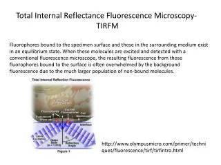
Total internal reflection fluorescence - TIRF: When total reflection appears, only an exponentially decaying evanescent wave crosses the interface only fluorophores close to the interface are excited ~ 3 – 300 nm
Total internal reflection fluorescence - TIRF: When total reflection appears, only an exponentially decaying evanescent wave crosses the interface only fluorophores close to the interface are excited prism-based objective-based
Confocal microscopy – Basic principle: A pinhole in the back focal plane rejects the light coming from outside the focal plane. The pinhole size is a trade-off between good rejecting ability and sufficient light throughput (typically ~ 30 – 150 mm) wide field confocal detection pinhole tube lens objective focal plane
Confocal microscopy – Basic principle: The pinhole restricts the observed volume of the sample to a single point (the size of which is restricted by the pinhole size). Excitation by a collimated beam (point source optically conjugated to the pinhole) focused to a diffraction limited spot wide field PMT MPD … confocal CCD image is scanned point by point dichroic whole image at once
Confocal microscopy – Scanning systems: spinning disk laser scanning microscope (LSM) • Collimated laser beam focus is scanned through the sample: • sample scanning by a piezo crystal • slow • possible combination with scanning probe microscopy (AFM, STM, …) • M. Petráň and M. Hadravský (1967) • Wide-filed illumination passes through pinholes in Nipkow disk (arranged in Archimedean spiral) • either a single pinhole for excitation and emission or 2 tandem disks • low excitation efficiency – only a small fraction of light passes pinhole beam scanning by a mirrors mounted on galvanometers • nowadays enhanced by microlens arrays on another Nipkow disk • more points in parallel possible – faster imaging X Y optical path for excitation and emission formed by the same mirrors Axial scanning (Z) usually by a piezo or stepper motor actuator
Confocal vs. Wide field microscopy: Wide-field: Confocal: Elimination of out-of-focus light improves contrast and, thus, resolution
Confocal vs. Wide field microscopy: Focusing only in one plane axial sectioning of the sample to ~ mm slices
Resolution in confocal microscopy: collimated laser beam is focused by the objective into a diffraction limited spot PSF (point spread function) = focus profile × collection efficiency of the objective. Those two are approximately the same diffraction limited spot. Slightly higher resolution than in wide field microscopy (improvement ~ 1.4) x ~ 200 nm z ~1 mm ~ 3D Gaussian profile The image is a convolution of the object and the PSF
single-photon excitation two-photon excitation h* h h Absorption Emission Emission Absorption h h* E = hn E ~ 1 / l E* = 1/2 E E* ~ 1 / 2l c = ln Two-photon microscopy – Basic idea: Two photons at the same time and at the same place with doubled wavelength • photons from the infra red spectrum (> 750 nm)– typically Ti:Sa laser • high photon density (6 – 7 orders of magnitude higher than in single photon confocal microscopy) • excitation probability proportional to I2 reduced detection volume, higher resolution(improvement mainly in axial direction, in lateral it can be negligible due to larger l)
photon non-excited dye molecule 2p-excited dye molecule Two-photon microscopy – Focus profile: laser pulse the required photon density for two-photon excitation can be established only in the focal plane no out-of focus fluorescence no pinhole needed focal plane 2p-excitation 1p-excitation
Two-photon microscopy: Advantages • improved axial resolution • reduced bleaching out of focus • higher light collection efficiency (no pinhole) • higher depth of light penetration • broader excitation spectra – simultaneous excitation of more dyes • Limitations • more costly and complicated instrumental setup • higher bleaching in the focus • broader excitation spectra – decreased selectivity of excitation • scanning technique like confocal microscopy
General features of scanning microscopy: Advantages • improved contrast • optical sectioning ability • possibility to perform fluorescence measurements in individual points (lifetime, spectra, FCS, …) • Limitations • more complicated and costly setup • limited speed of image acquisition • longer imaging more photobleaching Fluorescence lifetime imaging (FLIM)
Below the diffraction limit: • Going to near-field, where the diffraction limit does not hold – Near-field Scanning Optical Microscope (NSOM) • Effectively increasing the numerical aperture (does not really break the limit, but increases resolution) – Structured (Patterned) Illumination Microscopy (SIM), … • Localization of individual fluorophoresand fitting their PSFs, typically combined with switching between dark and fluorescent state (PALM, STORM, …); or utilizing intensity fluctuations of individual fluorophores (Superresolution Optical Fluctuation Imaging – SOFI) • Employing nonlinear optical effects: • Multi-photon excitation • Optical saturation – nonlinear dependence of fluorescence on excitation intensity, happens at high excitation intensities when large fraction of fluorophores resides in excited state and cannot be excited • Other saturation phenomena: Dynamic saturation optical microscopy (DSOM) – kinetics of transition to triplet state, Stimulated emission excited state depletion (STED)
Near-field scanning optical microscopy (NSOM): Diffraction limit is valid in the far-filed, where spherical wave-fronts exiting from an aperture can be regarded locally as plane waves – coming close to the sample changes the situation – scanning probe approach The probe – usually a metal coated tapered optical fibre moved by a piezo scanner various operation modes – purely near-field or combining near-/far-field excitation/emission or vice versa • resolution~ 20 nm in lateral (determined by tip size) and ~ 2-5 nm in axial direction • limited only to surfaces
Effective increasing of numerical aperture: 4Pi microscopy structured illumination • 2 opposing objectives – PSF closer to spherical symmetry – 3-7 times improved axial resolution (depends on type) • Sample is illuminated by a periodically modulated light. Interference of structures in the sample and illumination results in Moiré fringes • combination with nonlinear image restoration – improvement in 3D • a confocal approach - scanning • Additional spatial frequency increases the resolution power by factor 2 • A wide-field approach – faster then scanning • Several images with shifted illumination patterns are recorded and the final image is reconstructed by Fourier transform analysis optical sectioning
Localization of individual molecules: Single fluorophores have dimensions much smaller than the PSF. A single fluorophore is seen in the image as the PSF By fitting the PSF in the image with a Gaussian profile, fluorophore location can be determined with a few nm accuracy precise determination of distances, single particle tracking (SPT) Schmidt et al. (1996) PNAS 93:2926-2629
Localization of individual molecules: At higher densities of fluorophores, the PSFs overlap – impossible to distinguish the centers of peaks. Nevertheless, fluorophores need to be densely located in the sample to be cover to all structural details STORM – Stochastic optical reconstruction microscopy Rust et al. (2006) Nature Meth 3:793-795 • Uses photoswitchable dyes (special organic dyes, GFP mutants): • a strong red laser pulse switches off all fluorophores (to a nonfluorescent state) • a green laser pulse switches on a small fraction of fluorophores, which emit fluorescence when excited with red laser until switched off, cycle repeated … A wide field technique, but imaging slow because many imaging cycles needed Resolution ~ 20-30 nm PALM –Photoactivated localization microscopy the same principle with switching of dyes between on and off states
Optical saturation and resolution enhancement: Optical saturation results in nonlinear relation between excitation and fluorescence intensities broadening of the PSF We apply a ramp of excitation intensity and the dependence of fluorescence intensity in each pixel on excitation intensity can be fitted with a polynomial expansion Ifl(x,y) = Iex - Iex2 + Iex3 - Iex4... Theoretically unlimited resolution, but practically limited by noise and poor stability of polynomial fits (~ 30%) Saturated excitation microscopy (SAX) – harmonically modulated excitation, Saturated structured illumination (SSIM) – SIM combined with nonlinearity
Imax>> Isaturation Fluorescence STED pulse Excitation spot x ~ Stimulated emission excited state depletion (STED): Developed by Stefan Hell (http://www.mpibpc.mpg.de/abteilungen/200/STED.htm) • A confocal approach • Fluorophores in the detection volume are excited by an excitation pulse. • A doughnut-shaped STED pulse is applied, which suppresses the fluorescence completely (by inducing stimulated emission) everywhere except the center of the detection volume • Photons in STED pulse have lower energy to avoid excitation • STED pulse duration should be much shorter then S1 lifetime = 1/kfluor • Saturation of the stimulated emission in the STED pulse is essential for breaking the diffraction limit saturation parameter: x = I max/ Isaturation kIC >kSE>> kfluor
STED: Theoretically unlimited resolution, usually ~ 3 times in lateral and ~ 6 times in axial direction is achieved
Selective plane illumination microscopy: Based on q microscopy (uses excitation and detection optics at 90˚ instead of epi-fluorescence to generate isotropic PSF) – combination with light sheet illumination faster imaging of 3D objects http://www.lmg.embl.de/home.html
Acknowledgement The course was inspired by courses of: Prof. David M. Jameson, Ph.D. Prof. RNDr. Jaromír Plášek, Csc. Prof. William Reusch Financial support from the grant: FRVŠ 33/119970