Mining for Spatial Patterns
Mining for Spatial Patterns . Shashi Shekhar Department of Computer Science University of Minnesota http://www.cs.umn.edu/~shekhar Collaborators: V. Kumar, G. Karypis, C.T. Lu, W. Wu, Y. Huang, V. Raju, P. Zhang, P. Tan, M. Steinbach

Mining for Spatial Patterns
E N D
Presentation Transcript
Mining for Spatial Patterns Shashi Shekhar Department of Computer Science University of Minnesota http://www.cs.umn.edu/~shekhar Collaborators: V. Kumar, G. Karypis, C.T. Lu, W. Wu, Y. Huang, V. Raju, P. Zhang, P. Tan, M. Steinbach This work was partially funded by NASA and Army High Performance Computing Center Mining For Spatial Patterns
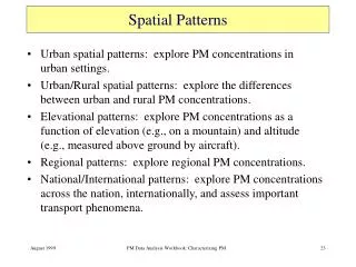
Spatial Data Mining(SDM) - Examples • Historical Examples: • London Asiatic Cholera 1854 (Griffith) • Dental health and fluoride in water, Colorado early 1900s • Current Examples: • Cancer clusters (CDC), Spread of disease (e.g. Nile virus) • Crime hotspots (NIJ CML, police petrol planning) • Environmental justice (EPA), fair lending practices • Upcoming Applications: Location aware services • Defense: Sensor networks, Mobile ad-hoc networks • Civilian: Mortgage PMI determination based on location Mining For Spatial Patterns
Army Relevance of SDM • Strategic • Predicting global hot spots (FORMID) • Army land: endangered species vs. training and war games • Search for local trends in massive simulation data • Critical infra-structure defense (threat assessment) • Tactical • Inferring enemy tactics (e.g. flank attack) from blobology • Detection of lost ammunition dumps (Dr. Radhakrishnan) • Operational • Interpretation of maps: map matching (locating oneself on map) • identify terrain feature, e.g. ravines, valleys, ridge, etc. • Locating enemy (e.g. sniper in a haystack, sensor networks) • Avoiding friendly fire Mining For Spatial Patterns
Spatial Data Mining(SDM) - Definition • Search of implicit, interesting patterns in geo-spatial data • Ex. Reconnaissance, Vector maps(NIMA, TEC), GPS, Sensor networks • Data Mining vs. Statistics: • Primary vs. Secondary analysis • Global vs. local trends • Spatial Data Mining vs. Data Mining: • Spatial Autocorrelation • Continuous vs. Discrete data types Mining For Spatial Patterns
Background • Spatial Data Mining • Spatial statistics in Geology, Regional Economics • NSF workshop on GIS and DM (3/99) • NSF workshop on spatial data analysis (5/02) • Spatial patterns: • Spatial outliers • Location prediction • Associations, colocations • Hotspots, Clustering, trends, … Mining For Spatial Patterns
Framework • 2 Approaches to mining Spatial Data • 1. Pick spatial features; use classical DM methods • 2. Use novel data mining techniques • Our Approach: • Define the problem: capture special needs • Explore data using maps, other visualization • Try reusing classical DM methods • If classical DM perform poorly, try new methods • Evaluate chosen methods rigourously • Performance tuning if needed Mining For Spatial Patterns
Spatial Association Rule • Citation: Symp. On Spatial Databases 2001 • Problem: Given a set of boolean spatial features • find subsets of co-located features, e.g. (fire, drought, vegetation) • Data - continuous space, partition not natural, no reference feature • Classical data mining approach: association rules • But, Look Ma! No Transactions!!! No support measure! • Approach: Work with continuous data without transactionizing it! • confidence = Pr.[fire at s | drought in N(s) and vegetation in N(s)] • support: cardinality of spatial join of instances of fire, drought, dry veg. • participation: min. fraction of instances of a features in join result • new algorithm using spatial joins and apriori_gen filters Mining For Spatial Patterns
Event Definition • Convert the time series into sequence of events at each spatial location. Mining For Spatial Patterns
Interesting Association Patterns • Use domain knowledge to eliminate uninteresting patterns. • A pattern is less interesting if it occurs at random locations. • Approach: • Partition the land area into distinct groups (e.g., based on land-cover type). • For each pattern, find the regions for which the pattern can be applied. • If the pattern occurs mostly in a certain group of land areas, then it is potentially interesting. • If the pattern occurs frequently in all groups of land areas, then it is less interesting. Mining For Spatial Patterns
Association Rules FPAR-Hi NPP-Hi (support 10) Shrubland regions • Intra-zone non-sequential Patterns • Region corresponds to semi-arid grasslands, a type of vegetation, which is able to quickly take advantage of high precipitation than forests. • Hypothesis: FPAR-Hi events could be related to unusual precipitation conditions. Mining For Spatial Patterns
Co-location Can you find co-location patterns from the following sample dataset? Answers: and Mining For Spatial Patterns
Co-location Spatial Co-location A set of features frequently co-located Given A set T of K boolean spatial feature types T={f1,f2, … , fk} A set P of N locations P={p1, …, pN } in a spatial frame work S, pi P is of some spatial feature in T A neighbor relation R over locations in S Find Tc = subsets of T frequently co-located Objective Correctness Completeness Efficiency Constraints R is symmetric and reflexive Monotonic prevalence measure Reference Feature Centric Window Centric Event Centric Mining For Spatial Patterns
Co-location Comparison with association rules Participation index Participation ratio pr(fi, c) of feature fi in co-location c = {f1, f2, …, fk}: fraction of instances of fi with feature {f1, …, fi-1, fi+1, …, fk} nearby 2.Participation index = min{pr(fi, c)} Algorithm Hybrid Co-location Miner Mining For Spatial Patterns
Spatial Co-location Patterns • Dataset • Spatial feature A,B,C and their instances • Possible associations are (A, B), (B, C), etc. • Neighbor relationship includes following pairs: • A1, B1 • A2, B1 • A2, B2 • B1, C1 • B2, C2 Mining For Spatial Patterns
Spatial Co-location Patterns • Dataset • Partition approach[Yasuhiko, KDD 2001] • Support not well defined,i.e. not independent of execution trace • Has a fast heuristic which is hard to analyze for correctness/completeness Spatial feature A,B, C, and their instances Support A,B=1 B,C=2 Support A,B =2 B,C=2 Mining For Spatial Patterns
Spatial Co-location Patterns • Dataset • Reference feature approach [Han SSD 95] • C as reference feature to get transactions • Transactions: (B1) (B2) • Support (A,B) = Ǿ from Apriori algorithm • Note: Neighbor relationship includes following pairs: • A1, B1 • A2, B1 • A2, B2 • B1, C1 • B2, C2 Spatial feature A,B, C, and their instances Mining For Spatial Patterns
Spatial Co-location Patterns • Dataset • Our approach (Event Centric) • Neighborhood instead of transactions • Spatial join on neighbor relationship • Support Prevalence • Participation index = min. p_ratio • P_ratio(A, (A,B)) = fraction of instance of A participating in join(A,B, neighbor) • Examples • Support(A,B)=min(2/2,3/3)=1 • Support(B,C)=min(2/2,2/2)=1 Spatial feature A,B, C, and their instances Mining For Spatial Patterns
Spatial Co-location Patterns • Partition approach • Our approach • Dataset Support(A,B)=min(2/2,3/3)=1 Spatial feature A,B, C, and their instances Support(B,C)=min(2/2,2/2)=1 Support A,B =2 B,C=2 • Reference feature approach C as reference feature Transactions: (B1) (B2) Support (A,B) = Ǿ Support A,B=1 B,C=2 Mining For Spatial Patterns
Spatial Outliers • Spatial Outlier: A data point that is extreme relative to it neighbors • Case Study: traffic stations different from neighbors [SIGKDD 2001, JIDA 2002] • Data - space-time plot, distr. Of f(x), S(x) • Distribution of base attribute: • spatially smooth • frequency distribution over value domain: normal • Classical test - Pr.[item in population] is low • Q? distribution of diff.[f(x), neighborhood agg{f(x)}] • Insight: this statistic is distributed normally! • Test: (z-score on the statistics) > 2 • Performance - spatial join, clustering methods Mining For Spatial Patterns
Spatial Outlier Detection Given A spatial graph G={V,E} A neighbor relationship (K neighbors) An attribute function : V -> R An aggregation function : :R k -> R A comparison function Confidence level threshold Statistic test function ST: R ->{T, F} Find O = {vi | vi V, vi is a spatial outlier} Objective Correctness: The attribute values of vi is extreme, compared with its neighbors Computational efficiency Constraints and ST are algebraic aggregate functions of and Computation cost dominated by I/O op. Mining For Spatial Patterns
Spatial Outlier Detection Spatial Outlier Detection Test 1. Choice of Spatial Statistic S(x) = [f(x)–E y N(x)(f(y))] Theorem: S(x) is normally distributed if f(x) is normally distributed 2. Test for Outlier Detection | (S(x) - s) / s | > Hypothesis I/O cost determined by clustering efficiency f(x) S(x) Mining For Spatial Patterns
Graphical Spatial Tests Moran Scatter Plot Original Data Variogram Cloud Mining For Spatial Patterns
A Unified Approach Spatial Outliers • Tests : quantitative, graphical • Results: • Computation = spatial self-join • Tests: algebraic functions of join • Join predicate: neighbor relations • I/O-cost: f(clustering efficiency) • Our algorithm is I/O-efficient for • Algebraic tests Scatter Plot Original Data Our Approach Mining For Spatial Patterns
Spatial Outlier Detection Results 1. CCAM achieves higher clustering efficiency (CE) 2. CCAM has lower I/O cost 3. High CE => low I/O cost 4. Big Page => high CE CE value I/O cost Z-order Cell-Tree CCAM Mining For Spatial Patterns
Location Prediction • Citations: IEEE Tran. on Multimedia2002, SIAM DM Conf. 2001, SIGKDD DMKD 2000 • Problem: predict nesting site in marshes • given vegetation, water depth, distance to edge, etc. • Data - maps of nests and attributes • spatially clustered nests, spatially smooth attributes • Classical method: logistic regression, decision trees, bayesian classifier • but, independence assumption is violated ! Misses auto-correlation ! • Spatial auto-regression (SAR), Markov random field bayesian classifier • Open issues: spatial accuracy vs. classification accurary • Open issue: performance - SAR learning is slow! Mining For Spatial Patterns
Location Prediction Given: 1. Spatial Framework 2. Explanatory functions: 3. A dependent class: 4. A family of function mappings: Find: Classification model: Objective:maximize classification_accuracy Constraints: Spatial Autocorrelation exists Nest locations Distance to open water Water depth Vegetation durability Mining For Spatial Patterns
Motivation and Framework Mining For Spatial Patterns
Spatial AutoRegression (SAR) • Spatial Autoregression Model (SAR) • y = Wy + X + • W models neighborhood relationships • models strength of spatial dependencies • error vector • Solutions • and - can be estimated using ML or Bayesian stat. • e.g., spatial econometrics package uses Bayesian approach using sampling-based Markov Chain Monte Carlo (MCMC) method. • Likelihood-based estimation requires O(n3) ops. • Other alternatives – divide and conquer, sparse matrix, LU decomposition, etc. Mining For Spatial Patterns
Evaluation • Linear Regression • Spatial Regression • Spatial model is better Mining For Spatial Patterns
MRF Bayesian • Markov Random Field based Bayesian Classifiers • Pr(li | X, Li) = Pr(X|li, Li) Pr(li | Li) / Pr (X) • Pr(li | Li) can be estimated from training data • Li denotes set of labels in the neighborhood of si excluding labels at si • Pr(X|li, Li) can be estimated using kernel functions • Solutions • stochastic relaxation [Geman] • Iterated conditional modes [Besag] • Graph cut [Boykov] Mining For Spatial Patterns
Experiment Design Mining For Spatial Patterns
Prediction Maps(Learning) Actual Nest Sites (Real Learning) MRF-P Prediction (ADNP=3.36) NZ=85 NZ=138 MRF-GMM Prediction (ADNP=5.88) SAR Prediction (ADNP=9.80) NZ=140 NZ=130 Mining For Spatial Patterns
Prediction Maps(Testing) Actual Nest Sites (Real Testing) MRF-P Prediction (ADNP=2.84) Actual Nest Sites (Real Learning) NZ=30 NZ=80 MRF-GMM Prediction (ADNP=3.35) SAR Prediction (ADNP=8.63) NZ=76 NZ=80 Mining For Spatial Patterns
Comparison (MRF-BC vs. SAR) • SAR can be rewritten as y = (QX) + Q • where Q = (I- W)-1 which can be viewed as a spatial smoothing operation. • This transformation shows that SAR is similar to linear logistic model, and thus suffers with same limitations – i.e., SAR model assumes linear separability of classes in transformed feature space • SAR model also make more restrictive assumptions about the distribution of features and class shapes than MRF • The relationship between SAR and MRF are analogous to the relationship between logistic regression and Bayesian classifiers. • Our experimental results shows that MRF model yields better spatial and classification accuracies than SAR predictions. Mining For Spatial Patterns
MRF vs. SAR Confusion Matrix: Spatial Confusion Matrix: Mining For Spatial Patterns
Conclusion and Future Directions • Spatial domains may not satisfy assumptions of classical methods • data: auto-correlation, continuous geographic space • patterns: global vs. local, e.g. spatial outliers vs. outliers • data exploration: maps and albums • Open Issues • patterns: hot-spots, blobology (shape), spatial trends, … • metrics: spatial accuracy(predicted locations), spatial contiguity(clusters) • spatio-temporal dataset • scale and resolutions sentivity of patterns • geo-statistical confidence measure for mined patterns Mining For Spatial Patterns
Army Relevance and Collaborations Relevance: “Maps are as important to soldiers as guns” - unknown Joint Projects: High Performance GIS for Battlefield Simulation (ARL Adelphi) Spatial Querying for Battlefield Situation Assessment (ARL Adelphi) Joint Publications: w/ G. Turner (ARL Adelphi, MD) & D. Chubb (CECOM IEWD) IEEE Computer (December 1996) IEEE Transactions on Knowledge and Data Eng. (July-Aug. 1998) Three conference papers Visits, Other Collaborations GIS group, Waterways Experimentation Station (Army) Concept Analysis Agency, Topographic Eng. Center, ARL, Adelphi Workshop on Battlefield Visualization and Real Time GIS (4/2000)
Reference • S. Shekhar, S. Chawla, S. Ravada, A. Fetterer, X. Liu and C.T. Liu, “Spatial Databases: Accomplishments and Research Needs”, IEEE Transactions on Knowledge and Data Engineering, Jan.-Feb. 1999. • S. Shekhar and Y. Huang, “Discovering Spatial Co-location Patterns: a Summary of Results”, In Proc. of 7th International Symposium on Spatial and Temporal Databases (SSTD01), July 2001. • S. Shekhar, C.T. Lu, P. Zhang, "Detecting Graph-based Spatial Outliers: Algorithms and Applications“, the Seventh ACM SIGKDD International Conference on Knowledge Discovery and Data Mining, 2001. • S. Shekhar, C.T. Lu, P. Zhang, “Detecting Graph-based Saptial Outlier”, Intelligent Data Analysis, To appear in Vol. 6(3), 2002 • S. Shekhar, S. Chawla, the book“Spatial Database: Concepts, Implementation and Trends”, Prentice Hall, 2002 • S. Chawla, S. Shekhar, W. Wu and U. Ozesmi, “Extending Data Mining for Spatial Applications: A Case Study in Predicting Nest Locations”, Proc. Int. Confi. on 2000 ACM SIGMOD Workshop on Research Issues in Data Mining and Knowledge Discovery (DMKD 2000), Dallas, TX, May 14, 2000. • S. Chawla, S. Shekhar, W. Wu and U. Ozesmi, “Modeling Spatial Dependencies for Mining Geospatial Data”, First SIAM International Conference on Data Mining, 2001. • S. Shekhar, P.R. Schrater, R. R. Vatsavai, W. Wu, and S. Chawla, “Spatial Contextual Classification and Prediction Models for Mining Geospatial Data”,To Appear in IEEE Transactions on Multimedia, 2002. • S. Shekhar, V. Kumar, P. Tan. M. Steinbach, Y. Huang, P. Zhang, C. Potter, S. Klooster, “Mining Patterns in Earth Science Data”, IEEE Computing in Science and Engineering (Submitted) Mining For Spatial Patterns
Reference • S. Shekhar, C.T. Lu, P. Zhang, “A Unified Approach to Spatial Outliers Detection”, IEEE Transactions on Knowledge and Data Engineering (Submitted) • S. Shekhar, C.T. Lu, X. Tan, S. Chawla, Map Cube: A Visualization Tool for Spatial Data Warehouses, as Chapter of Geographic Data Mining and Knowledge Discovery. Harvey J. Miller and Jiawei Han (eds.), Taylor and Francis, 2001, ISBN 0-415-23369-0. • S. Shekhar, Y. Huang, W. Wu, C.T. Lu, What's Spatial about Spatial Data Mining: Three Case Studies , as Chapter of Book: Data Mining for Scientific and Engineering Applications. V. Kumar, R. Grossman, C. Kamath, R. Namburu (eds.), Kluwer Academic Pub., 2001, ISBN 1-4020-0033-2 • Shashi Shekhar and Yan Huang , Multi-resolution Co-location Miner: a New Algorithm to Find Co-location Patterns in Spatial Datasets, Fifth Workshop on Mining Scientific Datasets (SIAM 2nd Data Mining Conference), April 2002 Mining For Spatial Patterns