
Deep Feedforward Networks
E N D
Presentation Transcript
Deep Feedforward Networks Hankz Hankui Zhuo May 10, 2019 http://xplan-lab.org
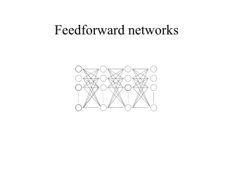
What’s DFN • Information flows through the function being evaluated from x, through the intermediate computations used to define f, and finally to the output y • No feedback connections • Extended to include feedback connections • RecurrentNeural Networks • Also called feedforward neural networks • Or multilayer perceptions (MLPs)
Structure • Chain structures: • three layers: f(x) = f3(f2(f1(x))) • “three” is the depth of the model • Output layer: the desired output is specified in the training data • Hidden layers: the desired output is not specified in the training data • Width of the model: the dimensionality of hidden layers
Mapping of input • Linear model of input x • y=wTx • Nonlinear model • Introducing mapping ϕ • y=wTϕ(x) • How to choose ϕ? • 1. use a very generic ϕ: • kernel machines, e.g., RBF kernel • If ϕ(x) is of high enough dimension, we can always have enough capacity to fit the training set • 2. manually engineer ϕ
Mapping of input • 3. The strategy of deep learning is to learn ϕ • y=f(x;θ,w)=ϕ(x; θ)Tw • This approach can capture the benefit of the first approach by being highly generic • we do so by using a very broad family φ(x;θ). • Can also capture the benefit of the second approach • Human practitioners can encode their knowledge to help generalization by designing families φ(x; θ) that they expect will perform well.
Example: Learning XOR • XOR is an operation on two binary values • When exactly one of these binary values is equal to 1, the XOR function returns 1 • Training data with four points • X={[0,0],[0,1],[1,0],[1,1]} • MSE (mean squared error) loss function: • J(θ)=1/4Σx(f(x)-f(x;θ))2 • Choose the form of our model f(x;θ) • Linear model: f(x;w,b)=xTw+b • We got w=0 and b=1/2, i.e., The linear model simply outputs 0.5 everywhere
Why? • When x1 = 0, the model’s output must increase as x2 increases. • When x1 = 1, the model’s output must decrease as x2 increases. • A linear model must apply a fixed coefficient w2 to x2. • The linear model therefore cannot use the value of x1 to change the coefficient on x2 and cannot solve this problem.
A simple feedforward network • One hidden layer with two hidden units • Hidden layer: • h = f1(x; W, c) • Output layer: • y=f2(h;w,b) • Complete model: • f(x;W,c,w,b)=f2(f1(x)) • If f1 use linear model, then • h=f1(x)=WTx, f2(h)=hTw, • Then we have y=f(x)=wTWTx • Or just f(x)=xTw’, where w’=Ww • We thus cannot solve the problem • We need a nonlinear function • Use a fixed nonlinear function called activation function • h=g(WTx+c) • g is typically chosen to be a function that is applied element-wise • hi=g(xTW:,i+ci)
Rectified Linear Unit (ReLU) • The activation function g is defined by • g(z)=max{0,z} • i.e., the complete network is: • f(x;W,c,w,b)=wTmax{0,WTx+c}+b
A solution to XOR • A solution as show below: • We can walk through the way the model processes based on f(x;W,c,w,b)=wTmax{0,WTx+c}+b apply ReLU add c multiply w
Gradient-Based Learning • difference between the linear models and neural networks is • the nonlinearity of a neural network causes most interesting loss functions to become non-convex • This means that neural networks are usually trained by using iterative, gradient-based optimizers that merely drive the cost function to a very low value, rather than the linear equation solvers used to train linear regression models or the convex optimization algorithms with global convergence guarantees • Stochastic gradient descent applied to non-convex loss functions has no such convergence guarantee, and is sensitive to the values of the initial parameters. • For feedforward neural networks, it is important to initialize all weights to small random values.
Gradient-Based Learning • The biases may be initialized to zero or to small positive values. • For the moment, it suffices to understand that the training algorithm is almost always based on using the gradient to descend the cost function in one way or another. • The specific algorithms are improvements and refinements on the ideas of gradient descent • Computing the gradient is slightly more complicated for a neural network, but can still be done efficiently and exactly
Cost Function • Cross-entropy between training data and the model distribution • The specific form of the cost function changes from model to model, depending on the specific form of logpmodel • For • We have
Output Units • suppose that the feedforward network provides a set of hidden features defined by • h = f(x;θ) • Linear Units for Gaussian Output Distributions • Maximizing the log-likelihood is then equivalent to minimizing the mean squared error
Output Units (continued) • Sigmoid Units for Bernoulli Output Distributions • Suppose we were to use a linear unit, and threshold its value to obtain a valid probability • A sigmoid output unit is defined by • logistic sigmoid
Output Units (continued) • The sigmoid output unit as having two components • First, it uses a linear layer to compute z=wTh+b • Next, it uses the sigmoid activation function to convert z into a probability • We omit the dependence on x for the moment to discuss how to define a probability distribution over y using the value z
Output Units (continued) • omit the dependence on x for the moment to discuss how to define a probability distribution over y using the value z • The sigmoid can be motivated by constructing an unnormalized probability distribution • We then normalize to see that this yields a Bernoulli distribution controlled by a sigmoidal transformation of z • The loss function for maximum likelihood learning of a Bernoulli parametrized by a sigmoid is