T utorial : U nderstanding the normal curve .

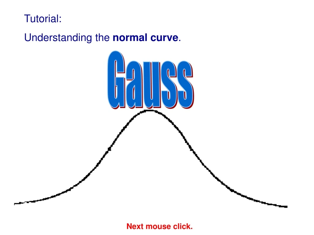
1. Gauss Tutorial: Understanding the normal curve. Next mouse click.

2. Standardizing Example Normal Distribution Standardized Normal Distribution

3. Standardize theNormal Distribution Normal Distribution Standardized Normal Distribution One table!

4. Infinite Number of Tables Normal distributions differ by mean & standard deviation. Each distribution would require its own table. That’s an infinite number!

5. We measure no. of visitors of 1000 portals and graph the results. The first portal has a 1000 visitors. We create a bar graph and plot that person on the graph. If our second portal has a 900 vistors, we add it to the graph. As we continue to plot portals, we create bell shape. 8 7 6 5 4 3 2 1 Number of Portsla withthat number of visitors Next mouse click 4 5 6 7 8 9 10 11 12 13 14 Number of visitors

6. Notice how there are more portals (n=6) with a 1000visitors than any other number of visitors. Notice also how as the numbr of visitors becomes larger or smaller, there are fewer and fewer portsla with that vistors number. This is a characteristics of many variables that we measure. There is a tendency to have most measurements in the middle, and fewer as we approach the high and low extremes. If we were to connect the top of each bar, we would create a frequency polygon. 8 7 6 5 4 3 2 1 Number of Portals with that number of visitors Next mouse click 4 5 6 7 8 9 10 11 12 13 14 Number of vistors

7. You will notice that if we smooth the lines, our data almost creates a bell shaped curve. 8 7 6 5 4 3 2 1 Number of Portsla 4 5 6 7 8 9 10 11 12 13 14 Number of visitors

8. You will notice that if we smooth the lines, our data almost creates a bell shaped curve. This bell shaped curve is known as the “Bell Curve” or the “Normal Curve.” 8 7 6 5 4 3 2 1 Number of Portals Next mouse click. 4 5 6 7 8 9 10 11 12 13 14 Number of visitors

9. 9 8 7 6 5 4 3 2 1 Number of Students 12 13 14 15 16 17 18 19 20 21 22 Points on a Quiz Sample of normal curve and the bar graph within it. Next mouse click.

10. 12 13 13 14 14 14 14 15 15 15 15 15 15 16 16 16 16 16 16 16 16 17 17 17 17 17 17 17 17 17 18 18 18 18 18 18 18 18 19 19 19 19 19 19 20 20 20 20 21 21 22 12+13+13+14+14+14+14+15+15+15+15+15+15+16+16+16+16+16+16+16+16+ 17+17+17+17+17+17+17+17+17+18+18+18+18+18+18+18+18+19+19+19+19+ 19+ 19+20+20+20+20+ 21+21+22 = 867 867 / 51 = 17 9 8 7 6 5 4 3 2 1 Number of Students 12 13 14 15 16 17 18 19 20 21 22 Points on a Quiz 12, 13, 13, 14, 14, 14, 14, 15, 15, 15, 15, 15, 15, 16, 16, 16, 16, 16, 16, 16, 16, 17, 17, 17, 17, 17, 17, 17, 17, 17, 18, 18, 18, 18, 18, 18, 18, 18, 19, 19, 19, 19, 19, 19, 20, 20, 20, 20, 21, 21, 22 The mean, mode, median Now lets look at quiz scores for 51 students.will all fall on the same value in a normal distribution. Your next mouse click will display a new screen.

11. Normal distributions (bell shaped) are a family of distributions that have the same general shape. They are symmetric (the left side is an exact mirror of the right side) with scores more concentrated in the middle than in the tails. Examples of normal distributions are shown to the right. Notice that they differ in how spread out they are. The area under each curve is the same. Next mouse click.

12. Mathematical Formula for Height of a Normal Curve The height (ordinate) of a normal curve is defined as: where m is the mean and s is the standard deviation, p is the constant 3.14159, and e is the base of natural logarithms and is equal to 2.718282.x can take on any value from -infinity to +infinity.f(x) is very close to 0 if x is more than three standard deviations from the mean (less than -3 or greater than +3). Next mouse click.

13. If your data fits a normal distribution, approximately 68% of your subjects will fall within one standard deviation of the mean. Approximately 95% of your subjects will fall within two standard deviations of the mean. Over 99% of your subjects will fall within three standard deviations of the mean. Next mouse click.

14. Assuming that we have a normal distribution, it is easy to calculate what percentage of students have z-scores between 1.5 and 2.5. To do this, use the Area Under the Normal Curve Calculator at http://davidmlane.com/hyperstat/z_table.html. Enter 2.5 in the top box and click on Compute Area. The system displays the area below a z-score of 2.5 in the lower box (in this case .9938) Next, enter 1.5 in the top box and click on Compute Area. The system displays the area below a z-score of 1.5 in the lower box (in this case .9332) If .9938 is below z = 2.5 and .9332 is below z = 1.5, then the area between 1.5 and 2.5 must be .9939 - .9332, which is .0606 or 6.06%. Therefore, 6% of our subjects would have z-scores between 1.5 and 2.5. Next mouse click.

15. Small Standard Deviation Large Standard Deviation Same Means Different Standard Deviations Different Means Same Standard Deviations Different Means Different Standard Deviations The mean and standard deviation are useful ways to describe a set of scores. If the scores are grouped closely together, they will have a smaller standard deviation than if they are spread farther apart. Click the mouse to view a variety of pairs of normal distributions below. Next mouse click.

16. When you have a subject’s raw score, you can use the mean and standard deviation to calculate his or her standardized score if the distribution of scores is normal. Standardized scores are useful when comparing a student’s performance across different tests, or when comparing students with each other. Your assignment for this unit involves calculating and using standardized scores. Next mouse click. z-score -3 -2 -1 0 1 2 3 T-score 20 30 40 50 60 70 80 IQ-score 65 70 85 100 115 130 145 SAT-score 200 300 400 500 600 700 800

17. On another test, a standard deviation may equal 5 points. If the mean were 45, then 68% of the students would score from 40 to 50 points. 30 35 40 45 50 55 60 Points on a Different Test The number of points that one standard deviations equals varies from distribution to distribution. On one math test, a standard deviation may be 7 points. If the mean were 45, then we would know that 68% of the students scored from 38 to 52. Next mouse click. • 31 38 45 52 59 63 • Points on Math Test

18. Because the tail is on the negative (left) side of the graph, the distribution has a negative (left) skew. Data do not always form a normal distribution. When most of the scores are high, the distributions is not normal, but negatively (left) skewed. Skew refers to the tail of the distribution. 8 7 6 5 4 3 2 1 Number of People with that Shoe Size Next mouse click. 4 5 6 7 8 9 10 11 12 13 14 Length of Right Foot

19. When most of the scores are low, the distributions is not normal, but positively (right) skewed. Because the tail is on the positive (right) side of the graph, the distribution has a positive (right) skew. 8 7 6 5 4 3 2 1 Number of People with that Shoe Size Your next mouse click will display a new screen. 4 5 6 7 8 9 10 11 12 13 14 Length of Right Foot

20. mean median mode mode median mean Negative or Left Skew Distribution Positive or Right Skew Distribution When data are skewed, they do not possess the characteristics of the normal curve (distribution). For example, 68% of the subjects do not fall within one standard deviation above or below the mean. The mean, mode, and median do not fall on the same score. The mode will still be represented by the highest point of the distribution, but the mean will be toward the side with the tail and the median will fall between the mode and mean. Your next mouse click will display a new screen.

21. The End Courtesy of University of Connecticut