An Adaptive Query Execution Engine for Data Integration

1. An Adaptive Query Execution Engine for Data Integration … Based on Zachary Ives, Alon Halevy & Hector Garcia-Molina’s Slides

2. Data Integration Systems Uniform query capability across autonomous, heterogeneous data sources on LAN, WAN, or Internet: in enterprises, WWW, big science.

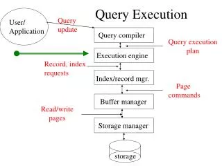
3. Traditional Query Processing SQL query parse parse tree convert answer logical query plan execute apply laws statistics Pi “improved” l.q.p pick best estimate result sizes {(P1,C1),(P2,C2)...} l.q.p. +sizes estimate costs consider physical plans {P1,P2,…..}

4. Example: SQL query SELECT title FROM StarsIn WHERE starName IN ( SELECT name FROM MovieStar WHERE birthdate LIKE ‘%1960’ ); (Find the movies with stars born in 1960)

5. Example: Logical Query Plan title starName=name  StarsIn name birthdate LIKE ‘%1960’ MovieStar

6. Example: Improved Logical Query Plan title starName=name StarsIn name birthdate LIKE ‘%1960’ MovieStar

7. Example: Estimate Result Sizes Need expected size StarsIn MovieStar P s

8. Example: One Physical Plan Parameters: join order, memory size, project attributes,... Hash join SEQ scan index scan Parameters: Select Condition,... StarsIn MovieStar

9. Example: (Grace) Hash Join • Hash function h, range 0  k • Buckets for R1: G0, G1, ... Gk • Buckets for R2: H0, H1, ... Hk Algorithm (Grace Hash Join) (1) Hash R1 tuples into G buckets (2) Hash R2 tuples into H buckets (3) For i = 0 to k do match tuples in Gi, Hi buckets Partitioning (steps 1—2); probing (step 3)

10. Simple example hash: even/odd R1 R2 Buckets R1 R2 2 5 Even: 4 4 3 12 Odd: 5 3 8 13 9 8 11 14 2 4 8 4 12 8 14 3 5 9 5 3 13 11

11. Hash Join Variations Question: what if there is enough memory to hold R1? R2 R1 5 4 12 3 13 8 11 14 2 4 3 5 8 9

12. Hash Join Variations Question: what if there is enough memory to hold R1? <5,5> • Load entire R1 into memory • (2) Build hash table for R1 • (using hash function h) • (2) For each tuple r2 in R2 do • - read r2 • - probe hash table for R1 using h(r2) • - for matching tuple r1, • output <r1,r2> 2, 4, 8 3, 5, 9 5 R1 hash table R2 R1 5 4 12 3 …

13. Example: Estimate costs L.Q.P P1 P2 …. Pn C1 C2 …. Cn Pick best!

14. New Challenges for Processing Queries in DI Systems • Little information for cost estimates • Unreliable, overlapping sources • Unpredictable data transfer rates • Want initial results quickly • Need “smarter” execution

15. The Tukwila Project • Key idea: build adaptive features into the core of the system • Interleave planning and execution (replan when you know more about your data) • Compensate for lack of information • Rule-based mechanism for changing behavior • Adaptive query operators: • Revival of the double-pipelined join  better latency • Collectors (a.k.a. “smart union”)  handling overlap

16. Tukwila Data Integration System Novel components: • Event handler • Optimization-execution loop

17. Handling Execution Events • Adaptive execution via event-condition-action rules • During execution, eventsgenerated Timeout, n tuples read, operator opens/closes, memory overflows, execution fragment completes, … • Events trigger rules: • Test conditions Memory free, tuples read, operator state, operator active, … • Execution actions Re-optimize, reduce memory, activate/deactivate operator, …

18. Interleaving Planning and Execution Re-optimize if at unexpected state: • Evaluate at key points, re-optimize un-executed portion of plan [Kabra/DeWitt SIGMOD98] • Plan has pipelined units, fragments • Send back statistics to optimizer. • Maintain optimizer state for later reuse. WHEN end_of_fragment(0) IF card(result) > 100,000 THEN re-optimize

19. Handling Latency Orders from data source A OrderNo 1234 1235 1399 1500 TrackNo 01-23-45 02-90-85 02-90-85 03-99-10 relation tuple attribute UPS from data source B TrackNo 01-23-45 02-90-85 03-99-10 04-08-30 Status In Transit Delivered Delivered Undeliverable SelectStatus = “Delivered” UPS Data from B often delayed due to high volume of requests

20. Join Operation Orders Need to combine tuples from Orders & UPS: OrderNo 1234 1235 1399 1500 TrackNo 01-23-45 02-90-85 02-90-85 03-99-10 JoinOrders.TrackNo = UPS.TrackNo(Orders, UPS) UPS OrderNo 1234 1235 1399 1500 TrackNo 01-23-45 02-90-85 02-90-85 03-99-10 Status In Transit Delivered Delivered Delivered TrackNo 01-23-45 02-90-85 03-99-10 04-08-30 Status In Transit Delivered Delivered Undeliverable (2nd TrackNo attribute is removed)

21. Query Plan Execution • Pipelining vs. materialization • Control flow? • Iterator (top-down) • Most common database model • Easier to implement • Data-driven (bottom-up) • Threads or external scheduling • Better concurrency Query plan represented as data-flow tree: “Show which orders have been delivered” JoinOrders.TrackNo = UPS.TrackNo SelectStatus = “Delivered” Read Orders Read UPS

22. Standard Hash Join Standard Hash Join • read entire inner • use outer tuples to probe inner hash table Double Pipelined Hash Join

23. Standard Hash Join • Standard hash join has 2 phases: • Non-pipelined: Read entire inner relation, build hash table • Pipelined: Use tuples from outer relation to probe the hash table • Advantages: • Only one hash table • Low CPU overhead • Disadvantages: • High latency: need to wait for all inner tuples • Asymmetric: need to estimate for inner • Long time to completion: sum of two data sources

24. Adaptive Operators: Double Pipelined Join Standard Hash Join Double Pipelined Hash Join • Hash table per source • As tuple comes in, add to hash table and probe opposite table

25. Double-Pipelined Hash Join <5,5> 2, 4 3, 5 5 probe store R1 hash table R2 hash table 5 5 (2) 5 arrives (1) 2,4,3,5 arrived R2 R1 4 12 3 … 8 9

26. Double-Pipelined Hash Join • Proposed for parallel main-memory databases (Wilschut 1990) • Advantages: • Results as soon as tuples received • Can produce results even when one source delays • Symmetric (do not need to distinguish inner/outer) • Disadvantages: • Require memory for two hash tables • Data-driven!

27. Double-Pipelined Join Adapted to Iterator Model • Use multiple threads with queues • Each child (A or B) reads tuples until full, then sleeps & awakens parent • DPJoin sleeps until awakened, then: • Joins tuples from QA or QB, returning all matches as output • Wakes owner of queue • Allows overlap of I/O & computation in iterator model • Little overlap between multiple computations DPJoin QA QB A B

28. Experimental Results(Joining 3 data sources) DPJoin Optimal Std Suboptimal Std Normal: DPJoin (yellow) as fast as optimal standard join (pink) Slow sources: DPJoin much better

29. Insufficient Memory? • May not be able to fit hash tables in RAM • Strategy for standard hash join • Swap some buckets to overflow files • As new tuples arrive for those buckets, write to files • After current phase, clear memory, repeat join on overflow files

30. Overflow Strategies • 3 overflow resolution methods: • Naive conversion — conversion into standard join; asymmetric • Flush left hash table to disk, pause left source • Read in right source • Pipeline tuples from left source • Incremental Left Flush — “lazy” version of above • As above, but flush minimally • When reading tuples from right, still probe left hash table • Incremental Symmetric Flush — remains symmetric • Choose same hash bucket from both tables to flush

31. Simple Algorithmic Comparison • Assume s tuples per source (i.e. sources of equal size), memory fits m tuples: • Left Flush: If m/2 < sm (only left overflows): Cost = 2(s - m/2) = 2s - m If m < s 2m (both overflow): Cost = 2(s + m2/2s - 3m/2) + 2(s - m) = 4s - 4m + m2/s • Symmetric Flush: If s < 2m: Cost = 2(2s - m) = 4s - 2m

32. Symmetric Increm. Left Naive Optimal (16MB) Experimental Results Low memory (4MB): symmetric as fast as optimal Medium memory (8MB): incremental left is nearly optimal • Adequate performance for overflow cases • Left flush consistent output; symmetric sometimes faster

33. Adaptive Operators: Collector Utilize mirrors and overlapping sources to produce results quickly • Dynamically adjust to source speed & availability • Scale to many sources without exceeding net bandwidth • Based on policy expressed via rules WHEN timeout(CustReviews) DO activate(NYTimes), activate(alt.books) WHEN timeout(NYTimes) DO activate(alt.books)

34. Summary • DPJoin shows benefits over standard joins • Possible to handle out-of-memory conditions efficiently • Experiments suggest optimal strategy depends on: • Sizes of sources • Amount of memory • I/O speed

35. The Unsolved Problem • Find interleaving points? When to switch from optimization to execution? • Some straightforward solutions worked reasonably, but student who was supposed to solve the problem graduated prematurely. • Some work on this problem: • Rick Cole (Informix) • Benninghoff & Maier (OGI). • One solution being explored: execute first and break pipeline later as needed. • Another solution: change operator ordering in mid-flight (Eddies, Avnur & Hellerstein).

36. More Urgent Problems • Users want answers immediately: • Optimize time to first tuple • Give approximate results earlier. • XML emerges as a preferred platform for data integration: • But all existing XML query processors are based on first loading XML into a repository.

37. Tukwila Version 2 • Able to transform, integrate and query arbitrary XML documents. • Support for output of query results as early as possible: • Streaming model of XML query execution. • Efficient execution over remote sources that are subject to frequent updates. • Philosophy: how can we adapt relational and object-relational execution engines to work with XML?

38. Tukwila V2 Highlights • The X-scan operator that maps XML data into tuples of subtrees. • Support for efficient memory representation of subtrees (use references to minimize replication). • Special operators for combining and structuring bindings as XML output.

39. Tukwila V2 Architecture

40. Example XML File <db> <book publisher="mkp"> <title>Readings in Database Systems</title> <editors> <name>Stonebraker</name> <name>Hellerstein</name> </editors> <isbn>123-456-X</isbn> </book><company ID="mkp"> <name>Morgan Kaufmann</title> <city>San Mateo</city> <state>CA</state> </company> </db>

41. XML Data Graph

42. Example Query WHERE <db> <book publisher=$pID> <title>$t</> </> ELEMENT_AS $b </> IN "books.xml", <db> <publication title=$t> <source ID=$pID>$p</> <price>$pr</> </> </> IN "amazon.xml", $pr < 49.95 CONSTRUCT <book> <name>$t</> <publisher>$p</> </>

43. Query Execution Plan

44. X-Scan • The operator at the leaves of the plan. • Given an XML stream and a set of regular expressions – produces a set of bindings. • Supports both trees and graph data. • Uses a set of state machines to traverse match the patterns. • Maintains a list to unseen element Ids, and resolves them upon arrival.

45. X-scan Data Structures

46. State Machines for X-scan

47. Other Features of Tukwila V.2 • X-scan: • Can also be made to preserve XML order. • Careful handling of cycles in the XML graph. • Can apply certain selections to the bindings. • Uses much of the code of Tukwila I. • No modifications to traditional operators. • XML output producing operators. • Nest operator.

48. In the “Pipeline” • Partial answers: no blocking. Produce approximate answers as data is streaming. • Policies for recovering from memory overflow [More Zack]. • Efficient updating of XML documents (and an XML update language) [w/Tatarinov] • Dan Suciu: a modular/composable toolset for manipulating XML. • Automatic generation of data source descriptions (Doan & Domingos)

49. First 5 Results

50. Completion Time