Download
1 / 1
10 likes | 164 Vues
This study evaluates the effectiveness of two methods—Edge Detection and Active Contour—for automating ice thickness estimation from polar subsurface radar imagery. Conducted by researchers from the Center for Remote Sensing of Ice Sheets and Elizabeth City State University, the work highlights how Active Contour effectively removes non-continuous plotted pixels, while the Edge Detection method excels in accurately identifying bedrock interfaces. Understanding these methods will enhance ice sheet studies and contribute to improved monitoring of climate change impacts.

E N D
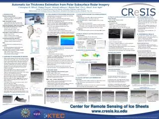
Pixel Column EDGE METHOD VS. CONTOUR METHOD ACTIVE CONTOUR CONFIGURATION Automatic Ice Thickness Estimation from Polar Subsurface Radar ImageryChristopher M. Gifford1, Gladys Finyom1, Michael Jefferson1, MyAsia Reid1, Eric L. Akers2, Arvin Agah11Center for Remote Sensing of Ice Sheets, University of Kansas, Lawrence, KS2Mathematics and Computer Science Department, Elizabeth City State University, Elizabeth City, NC Active Contour method rids the echogram of non-continuous plotted pixels Plotted points above the bedrock Artifact/noise in the bedrock layer Edge-detection method works better NASA/Rob Simmon • I. INTRODUCTION • Remote sensing methods: • CReSIS uses radar and seismic to acquire subsurface data from a remote location (i.e., surface, air, or space) • Radar and seismic sensors: • Used to gather data about the internal and bottom layers of ice sheets, from the surface • Surfaced and airborne radio echo sounding of Greenland and Antarctica ice sheets: • Determine ice sheets thickness • Bedrock topography (smooth, rough) • Mass balance of large bodies of ice • Challenges in radar sounding ice sheets: • Rough surface interface • Stages of melting (surface, internal) • Variations of ice thickness and topography • Processing subsurface radar data: • Requires knowledge about sensing medium • Ultimately used for scientific community • Goal: • Automating task of estimating ice thickness • Process: • Accurately selecting ice sheet’s surface, and interface between the ice and bedrock • Knowing surface, bedrock in radar imagery: • Helps compute the ice thickness • Helps ice sheet studies, their volume, and how they contribute to climate change • VI. EDGE DETECTION AND FOLLOWING APPROACH Introduction: • Edge detection, thresholding, edge connecting and following • [Assumption] Surface is max value in each trace • [Assumption] Bedrock is deepest contiguous layer in image Similar Work: • Skyline detector and segmentation: • Grow “seeds” from low variance sections in image sky regions • Seed regions reach image edge or threshold horizon found • Identify week clouds in Mars Exploration Rover sky imagery Our Approach: • Traces processed in bottom-up fashion until strong edge is found • III. CHALLENGES OF PROCESSING RADAR DATA • Automated processing and extraction of high level information from radar imagery is challenging • Clutter contributes to incomprehensible image regions • Bed topography varies from trace to trace due to rough bedrock interfaces from extended flight segments • A strong surface reflection can be repeated with an identical shape in an image, called a surface multiple, due to energy reflecting off the ice sheet surface and back again • Faint or non-existent bedrock reflections occur from: • Specific radar settings • Rough surface and bedrock topography • Presence of water on top of or internal to the ice sheet • These aspects produce gaps in the bedrock reflection layer which must be connected to construct a continuous layer for complete ice thickness estimation Greenland ice sheet Figure: Example contour adaptation sequence throughout processing, illustrating how the contour adapts to the bedrock interface and fits itself to the most salient edge near the bottom of the image Gap in bedrock Contour method bridges the gap • II. OVERVIEW OF RADAR REMOTE SENSING • Radars transmit energy in form of a pulse from an antenna, energy reflects off of targets, and is received by an antenna • Distance measured based on energy travel time back from targets (target reflection intensity and depth information) • Ground Penetrating Radar able to observe properties of subsurface, ranging from soil, sand, rock, snow, and ice • Energy from the radar into the ice changes in dielectric properties (air to ice, ice to bed rock) and causes the energy to reflect back • Water surrounded by the ice, and frozen ice against the bedrock both represent strong reflecting interfaces • Targets are internal layering in the ice sheets, and a strong echo return from bedrock beneath the ice • Interface below the surface (3.5 km or deeper) requires great transmit power and sensitive receive equipment because of energy loss within ice and with depth • Each measurement is called a radar trace, consisting of signals representing energy due to time (larger time deeper reflections) • In an image, a trace is an entire column of pixels, where each pixel represents a depth • Each row corresponds to a depth and time for a measurement, as the depth increases further down • A flight segment , called an echogram, consist of a collection of traces which represent all the columns of the image, from the beginning (left) to the end (right) • A pixel width represents the track distance between traces, and depends on the speed of the aircraft during the survey AUTOMATIC SURFACE & BOTTOM LAYER SELECTION Surface Selection: Same as Edge Detection method Bottom Selection: Data preprocessing EdgeCosts = 1/√(1+Gradient Magnitude) Create Image Gradient for upward force Add the edge cost image and upward force image • VIII. EXPERIMENTAL SETUP • Both methods implemented in Matlab • Data were 15 random subsets of 75 extended flights from Greenland (May and June 2006) • Range from 800-3000 rows and 1750-14500 columns (traces) • Previous manual selection method took ~45 minutes per file with ~7500 columns per file • Automated edge-based method takes ~15 seconds per file • Active contour (snake) method takes ~2.5 minutes per file • IX. EXPERIMENTAL RESULTS • Assumed human selections 100% accurate • Automatic selection is considered correct if it is within 5% of the human selection • There are several drawbacks with the manual approach (e.g., tired, inconsistent, interpolate) • EDGE-BASED METHOD • This method differs slightly from the active contour results even though both used general gradient magnitude technique • No continuity aspect causes method to suffer • ACTIVE CONTOUR METHOD • Method outperforms edge-based method • Drawback: takes longer to process images • Smooth and continuous aspects beneficial Plotted pixels below actual bedrock • AUTOMATIC SURFACE & BOTTOM LAYER SELECTION Surface Selection: • Extracting the location of the ice sheet surface • The depth corresponding to the max value of each trace is selected as location of surface reflection Bottom Selection: • Preprocessed by: • Detrending • Low-pass filtering • Contrast adjustment Figure: Edge cost image, enforcing low cost for strong edges and high cost for noise regions Figure: Combined edge cost and upward cost images • Contour initialization procedure • The contour is allowed to adapt until it reaches equilibrium • 2N+1 window (N = 50 pixels) is maintained • Window utilized for computing local stiffness to instill continuity and smoothness during adjustment • Determine lowest cost (0) pixels and highest cost (1) pixels • Allows contour to fit to the bedrock layer and bridge faint gaps Figure shows CReSIS picking software, the surface return is fully picked, while bedrock return is partially picked. Figure: Echogram that has been preprocessed using detrending, low-pass filter, and contrast enhancement Figure: Normalized echogram gradient magnitude, showing the image edges • IV. ICE THICKNESS ESTIMATION FROM RADAR • Ice thickness is needed for scientists to: • Study mass balance • Sea level rise • Environmental and human impacts • Ice thickness is computed by selecting the surface and bedrock reflections in pixel/depth coordinates, for each trace, and subtracting their corresponding depths • Several experts were utilized to manually select layers (time) • Surface selected based on the first and largest reflection return • Bedrock more challenging due to being possibly buried in noise • Experts tend to skip traces (e.g., 40 between selections) to speed up the process • Causes errors and inconsistencies which vary over time • Thousands of images manual approach becomes impractical 2D DERIVATIVE OF GAUSSIAN KERNEL CONTOUR COST WINDOW EXAMPLE RADAR ECHOGRAM: GREENLAND 05/28/2006 Figure: 2D derivative of Gaussian convolution kernels (1.5 ) for computing vertical (left) and horizontal (right) image gradients. CLEANED EDGE IMAGE & RESULT IMAGE Figure shows radar echogram over an ice sheet, illustrating the reflection of internal layers and the bedrock interface beneath the ice sheet. Figure: contour stiffness cost window during processing (left) for the contour’s configuration during the 75th iteration (right), illustrating how the contour is encouraged to make smooth transitions from trace-to-trace. CONTOUR ADJUSTMENT TotalCostWindow(t) = EdgeCosts(s) + α x UpwardCosts(t) + β x ContourStiffnessCosts(t) The lowest cost pixel location at each trace is selected as the contour’s next configuration If configuration does not change between iterations, or 500 iterations have been processed, the contour is determined to have reached equilibrium Ice thickness is computed for each trace by converting pixels for the bedrock selection to a depth in meters and subtracting it from the surface depth • V. RELATED WORK • Finding / Following Ice Sheet Internal Layers: • Predicts depth in certain layers • Focus on the Eemian Layer in Greenland ice sheet • Utilized Monte Carlo Inversion flow model to estimate unknown parameters guided by internal layers Edge / Layer / Contour Identification: • Layers, contours, and curves are discovered using image processing and computer vision methods • Adaptive contour (snake) fitting, where an image is a cost grid and the contour properties are measured as energy • Medical imagery (MRIs and CAT scans) Figure: Echogram with overlaid automatically selected surface (top, red) and bedrock (middle, blue) layers using the active contour method. Green is the initial contour. Reflection intensities are strongest at the surface and weaker because of depth. Depth increases from left to right. Figure: Cleaned edge image following thresholding, morphological closing and thinning operations Figure: Echogram with overlaid automatically selected surface (top, red) and bedrock (middle, blue) layers using the edge-based method. Four outlet Glaciers studied by CReSIS researchers. Leigh Stearns • VII. ACTIVE CONTOUR, COST MINIMIZATION • Similar Work: • Mars Exploration Rovers (MER) automatic sky segmentation system • Image segmentation (watershed and level set methods) • Our Approach: • Adaptive contour technique to fit a continuous contour to the bedrock • layer using image and contour properties as costs HUMAN EXPERT VS. EDGE METHOD VS. ACTIVE CONTOUR METHOD Zoomed Section